Marginal effects / slopes, contrasts, means and predictions with broom.helpers

Terminology

The overall idea of “marginal effects” is too provide tools to better interpret the results of a model by estimating several quantities at the margins. However, it has been implemented in many different ways by different ways and there is a bunch of quasi-synonyms for the idea of “marginal effects”: statistical effects, marginal effects, marginal means, contrasts, marginal slopes, conditional effects, conditional marginal effects, marginal effects at the mean, and many other similarly-named ideas.

In broom.helpers, we tried to adopt a terminology consistent with the {marginaleffects} package, first released in September 2021, and with Andrew Heiss’ Marginalia blog post published in May 2022.

Adjusted Predictions correspond to the outcome predicted by a fitted model on a specified scale for a given combination of values of the predictor variables, such as their observed values, their means, or factor levels (a.k.a. “reference grid”). When prediction are averaged according to a specific regressor, we will then refer to Marginal Predictions.

Marginal Contrasts are referring to a comparison (e.g. difference) of the outcome for a certain regressor, considering “meaningfully” or “typical” values for the other predictors (at the mean/mode, at custom values, averaged over observed values…). Contrasts could be computed for categorical variables (e.g. difference between two specific levels) or for continuous variables (change in the outcome for a certain change of the regressor).

Marginal Effects / Slopes are defined for continuous variables as a partial derivative (slope) of the regression equation with respect to a regressor of interest. Put differently, the marginal effect is the slope of the prediction function, measured at a specific value of the regressor of interest. In scientific practice, the marginal effects fall in the same toolbox as the marginal contrasts.

Marginal Means are adjusted predictions of a model, averaged across a “reference grid” of categorical predictors. They are similar to marginal predictions, but with subtle differences.

broom.helpers embed several custom tidiers to compute such quantities and to return a tibble compatible with tidy_plus_plus() and all others broom.helpers’s tidy_*() function. Therefore, it is possible to produce nicely formatted tables with gtsummary::tbl_regression() or forest plots with ggstats::ggcoef_model().

Data preparation

Let’s consider the trial dataset from the gtsummary package and build a logistic regression model with two categorical predictors (trt and stage) and two continuous predictor (marker and age). We will include an interaction between trt and marker and polynomial terms for age (i.e. age and age^2).

library(broom.helpers)
library(gtsummary)
library(dplyr)
d <- trial |>
  filter(complete.cases(response, trt, marker, grade, age))

mod <- glm(
  response ~ trt * marker + stage + poly(age, 2),
  data = d,
  family = binomial
)
mod |>
  tbl_regression(
    exponentiate = TRUE,
    label = list(age = "Age in years")
  ) |>
  bold_labels()

Characteristic	OR¹	95% CI¹	p-value
Chemotherapy Treatment
Drug A	—	—
Drug B	1.08	0.40, 2.98	0.9
Marker Level (ng/mL)	1.26	0.73, 2.17	0.4
T Stage
T1	—	—
T2	0.44	0.17, 1.10	0.084
T3	0.85	0.33, 2.18	0.7
T4	0.66	0.26, 1.65	0.4
Age in years
Age in years	41.7	0.50, 4,791	0.11
Age in years²	1.04	0.01, 94.1	>0.9
Chemotherapy Treatment * Marker Level (ng/mL)
Drug B * Marker Level (ng/mL)	1.25	0.59, 2.68	0.6
¹ OR = Odds Ratio, CI = Confidence Interval

Marginal Predictions

Marginal Predictions at the Mean

A first approach to better understand / interpret the model consists to predict the value of a regressor, on the model scale, at “typical values” of the other regressors. The estimates are therefore easier to interpret, as they are expressed on the the scale of the outcome (here, for a binary logistic regression, as probabilities). The differences observed between the predictions at different modalities will depend only on the “effect” of that regressor as the others regressors will be fixed at the same “typical values”. However, all packages do not use the same definition of “typical values”.

the `{effects}`’s approach

The effects package offer an effects::Effect() function to compute marginal predictions at typical values. Although the function is named Effect(), the produced estimates are marginal predictions according to the terminology presented at the beginning of this vignette.

library(effects, quietly = TRUE)
#> lattice theme set by effectsTheme()
#> See ?effectsTheme for details.
e <- Effect("stage", mod)
e
#> 
#>  stage effect
#> stage
#>        T1        T2        T3        T4 
#> 0.3866154 0.2179846 0.3501056 0.2938566
plot(e)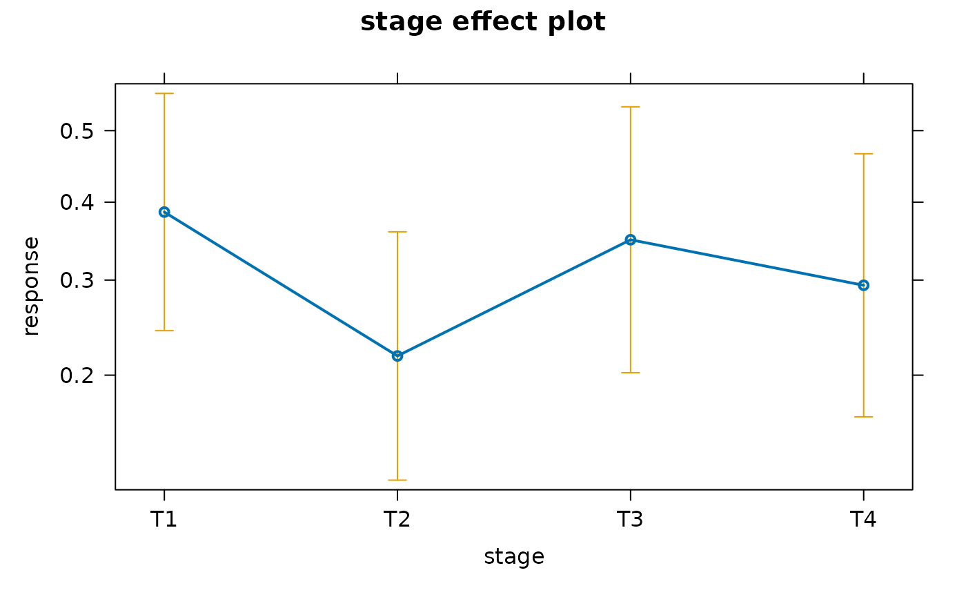

To understand what are the “typical values” used by effects::Effect(), let’s have a look at the model matrix generated by the package and used for predictions.

e$model.matrix
#>   (Intercept) trtDrug B    marker stageT2 stageT3 stageT4 poly(age, 2)1
#> 1           1 0.5202312 0.9191792       0       0       0 -2.228704e-16
#> 2           1 0.5202312 0.9191792       1       0       0 -2.228704e-16
#> 3           1 0.5202312 0.9191792       0       1       0 -2.228704e-16
#> 4           1 0.5202312 0.9191792       0       0       1 -2.228704e-16
#>   poly(age, 2)2 trtDrug B:marker
#> 1   -0.05568232        0.4781857
#> 2   -0.05568232        0.4781857
#> 3   -0.05568232        0.4781857
#> 4   -0.05568232        0.4781857
#> attr(,"assign")
#> [1] 0 1 2 3 3 3 4 4 5
#> attr(,"contrasts")
#> attr(,"contrasts")$trt
#> [1] "contr.treatment"
#> 
#> attr(,"contrasts")$stage
#> [1] "contr.treatment"

The other continuous regressors are set to their observed mean while the other categorical regressors are weighted according to their observed proportions. Somehow, an artificial “averaged” individual is created, of mean age and mean marker level, and being partly receiving Drug A and Drug B. And then, we predict the probability of response if this individual would be in stage T1, T2, T3 or T4.

For a continuous variable, effects::Effect() will consider several values of the regressor (based on the range of observed values) to estimate marginal predictions at these different values.

e2 <- Effect("age", mod)
e2
#> 
#>  age effect
#> age
#>         6        30        40        60        80 
#> 0.1664397 0.2392447 0.2760557 0.3606351 0.4568567
plot(e2)

The effects::allEffects() will build all marginal predictions of all regressors, taking into account eventual interactions within the model.

allEffects(mod)
#>  model: response ~ trt * marker + stage + poly(age, 2)
#> 
#>  stage effect
#> stage
#>        T1        T2        T3        T4 
#> 0.3866154 0.2179846 0.3501056 0.2938566 
#> 
#>  age effect
#> age
#>         6        30        40        60        80 
#> 0.1664397 0.2392447 0.2760557 0.3606351 0.4568567 
#> 
#>  trt*marker effect
#>         marker
#> trt          0.005         1         2         3         4
#>   Drug A 0.2338204 0.2776269 0.3264017 0.3792467 0.4351208
#>   Drug B 0.2479065 0.3408371 0.4484189 0.5610548 0.6677329
plot(allEffects(mod))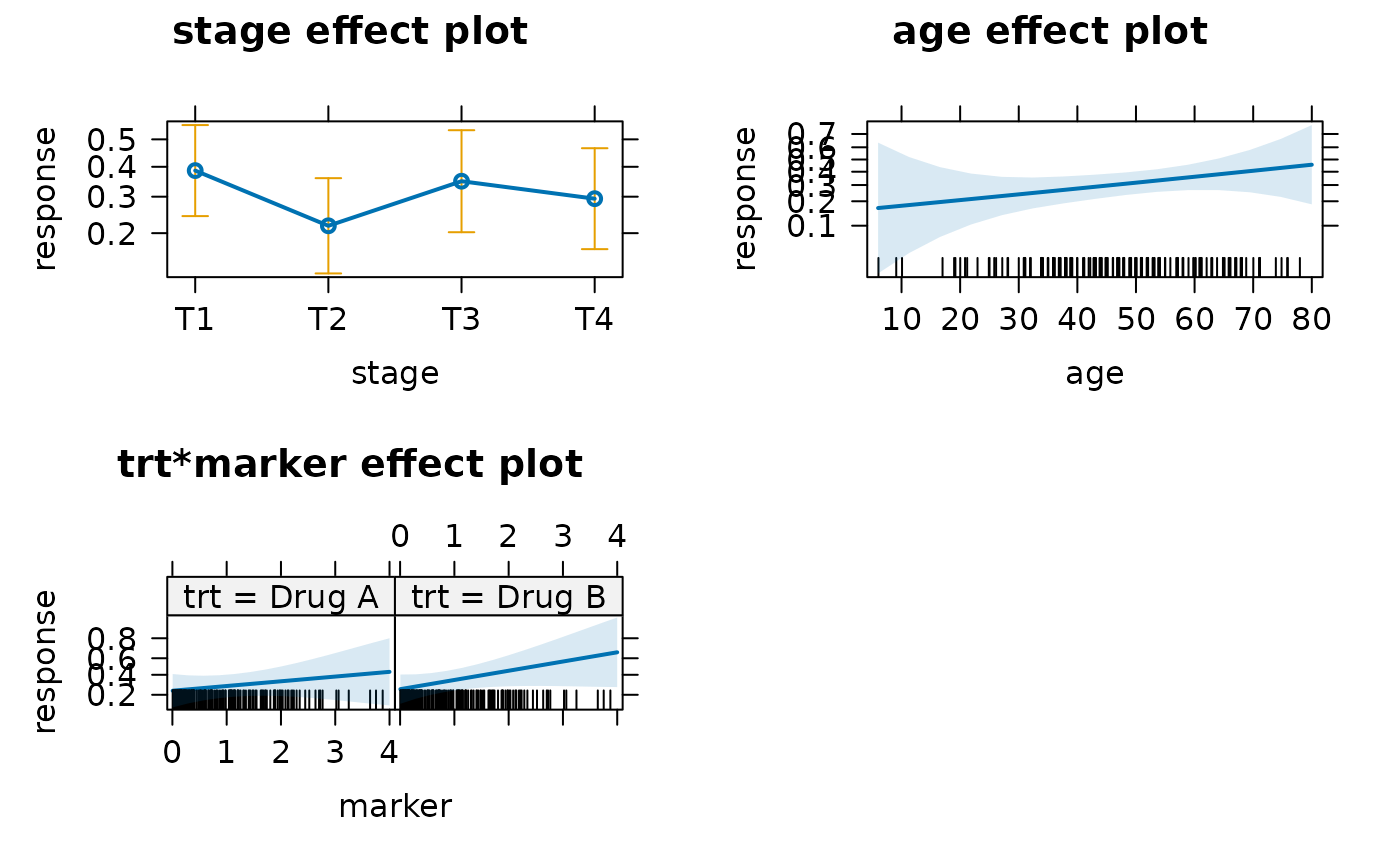

It is also possible to generate similar plots with ggeffects::ggeffect(). Please note that ggeffects::ggeffect() will consider, by default, only individual variables from the model and not existing interactions.

mod |>
  ggeffects::ggeffect() |>
  lapply(plot) |>
  patchwork::wrap_plots()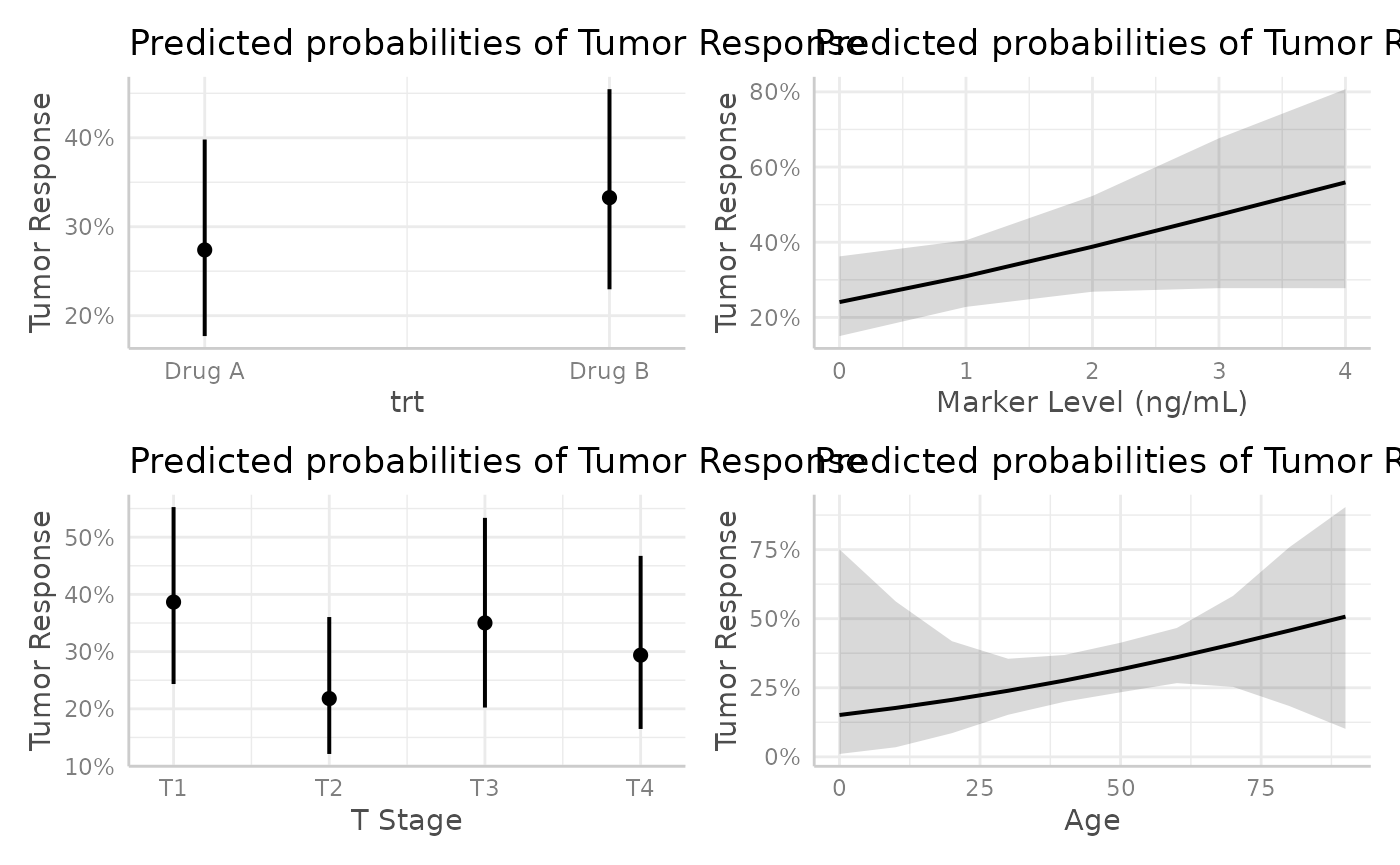

To generate a tibble of these results formatted in a way that it could be use with tidy_plus_plus() and other broom.helpers’s tidy_*() helpers, broom.helpers provides a tidy_all_effects() tieder.

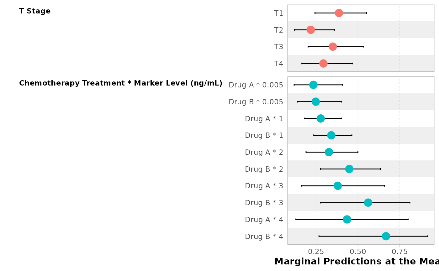
tidy_all_effects(mod)
#>       variable         term  estimate  std.error   conf.low conf.high
#> 1        stage           T1 0.3866154 0.08138561 0.24338626 0.5525749
#> 2        stage           T2 0.2179846 0.06122617 0.12116925 0.3604304
#> 3        stage           T3 0.3501056 0.08749758 0.20225147 0.5337316
#> 4        stage           T4 0.2938566 0.07895328 0.16486445 0.4673012
#> 5  poly(age,2)            6 0.1664397 0.15368239 0.02226625 0.6364570
#> 6  poly(age,2)           30 0.2392447 0.05197357 0.15232129 0.3549982
#> 7  poly(age,2)           40 0.2760557 0.04346297 0.19934983 0.3686854
#> 8  poly(age,2)           60 0.3606351 0.05152656 0.26686307 0.4663957
#> 9  poly(age,2)           80 0.4568567 0.16663622 0.18404077 0.7582667
#> 10  trt:marker Drug A:0.005 0.2338204 0.07478345 0.11867604 0.4088555
#> 11  trt:marker Drug B:0.005 0.2479065 0.06818623 0.13864532 0.4029880
#> 12  trt:marker     Drug A:1 0.2776269 0.05673207 0.18083471 0.4008740
#> 13  trt:marker     Drug B:1 0.3408371 0.05901662 0.23605720 0.4638846
#> 14  trt:marker     Drug A:2 0.3264017 0.08136674 0.19002540 0.5002087
#> 15  trt:marker     Drug B:2 0.4484189 0.09615134 0.27508336 0.6352624
#> 16  trt:marker     Drug A:3 0.3792467 0.13846045 0.16171930 0.6592599
#> 17  trt:marker     Drug B:3 0.5610548 0.15197028 0.27607502 0.8107519
#> 18  trt:marker     Drug A:4 0.4351208 0.20665349 0.12910815 0.8000955
#> 19  trt:marker     Drug B:4 0.6677329 0.19316496 0.26727889 0.9171600

It is therefore very easy to produce a nicely formatted table with gtsummary::tbl_regression() or a forest plot with ggstats::ggcoef_model().

mod |>
  tbl_regression(
    tidy_fun = tidy_all_effects,
    estimate_fun = scales::label_percent(accuracy = .1)
  ) |>
  bold_labels()

Characteristic	Marginal Predictions at the Mean	95% CI¹
T Stage
T1	38.7%	24.3%, 55.3%
T2	21.8%	12.1%, 36.0%
T3	35.0%	20.2%, 53.4%
T4	29.4%	16.5%, 46.7%
Chemotherapy Treatment * Marker Level (ng/mL)
Drug A * 0.005	23.4%	11.9%, 40.9%
Drug B * 0.005	24.8%	13.9%, 40.3%
Drug A * 1	27.8%	18.1%, 40.1%
Drug B * 1	34.1%	23.6%, 46.4%
Drug A * 2	32.6%	19.0%, 50.0%
Drug B * 2	44.8%	27.5%, 63.5%
Drug A * 3	37.9%	16.2%, 65.9%
Drug B * 3	56.1%	27.6%, 81.1%
Drug A * 4	43.5%	12.9%, 80.0%
Drug B * 4	66.8%	26.7%, 91.7%
¹ CI = Confidence Interval

ggstats::ggcoef_model(
  mod,
  tidy_fun = tidy_all_effects,
  vline = FALSE
)

the `{marginaleffects}`’s approach at the Mean

The marginaleffects package allows to compute marginal predictions “at the mean”, i.e. by considering the mean of the other continuous regressors and the mode (i.e. the most frequent observed modality) of categorical regressors. For that, we should call marginaleffects::predictions() with newdata = "mean".

library(marginaleffects)
predictions(
  mod,
  variables = "stage",
  newdata = "mean",
  by = "stage"
)
#> 
#>  stage Estimate Pr(>|z|)   S 2.5 % 97.5 %
#>     T1    0.419  0.39097 1.4 0.254  0.604
#>     T2    0.242  0.00282 8.5 0.131  0.403
#>     T4    0.322  0.06889 3.9 0.176  0.514
#>     T3    0.381  0.24194 2.0 0.215  0.581
#> 
#> Columns: stage, estimate, p.value, s.value, conf.low, conf.high 
#> Type:  invlink(link)

Four “mean individuals” were generated, with just the value of stage being different from one individual to the other, before predicting the probability of response.

For a continuous variable, predictions will be made, by default, at Tukey’s five numbers, i.e. the minimum, the first quartile, the median, the third quartile and the maximum.

predictions(
  mod,
  variables = "age",
  newdata = "mean",
  by = "age"
)
#> 
#>  age Estimate Pr(>|z|)    S  2.5 % 97.5 %
#>    6    0.127  0.10655  3.2 0.0139  0.602
#>   37    0.208  < 0.001 10.2 0.1072  0.365
#>   47    0.242  0.00286  8.5 0.1310  0.403
#>   57    0.280  0.01347  6.2 0.1550  0.451
#>   83    0.395  0.62840  0.7 0.1042  0.786
#> 
#> Columns: age, estimate, p.value, s.value, conf.low, conf.high 
#> Type:  invlink(link)

broom.helpers provides a global tidier tidy_marginal_predictions() to compute the marginal predictions for each variable or combination of variables before stacking them in a unique tibble. You should specify newdata = "mean" to get marginal predictions at the mean. By default, as effects::allEffects(), it will consider all higher order combinations of variables (as identified with model_list_higher_order_variables()).

mod |>
  model_list_higher_order_variables()
#> [1] "stage"      "age"        "trt:marker"
mod |>
  tbl_regression(
    tidy_fun = tidy_marginal_predictions,
    newdata = "mean",
    estimate_fun = scales::label_percent(accuracy = .1),
    label = list(age = "Age in years")
  ) |>
  modify_column_hide("p.value") |>
  bold_labels()

Characteristic	Marginal Predictions at the Mean	95% CI¹
T Stage
T1	41.9%	25.4%, 60.4%
T2	24.2%	13.1%, 40.3%
T3	38.1%	21.5%, 58.1%
T4	32.2%	17.6%, 51.4%
Age in years
6	12.7%	1.4%, 60.2%
37	20.8%	10.7%, 36.5%
47	24.2%	13.1%, 40.3%
57	28.0%	15.5%, 45.1%
83	39.5%	10.4%, 78.6%
Chemotherapy Treatment * Marker Level (ng/mL)
Drug A * 0.005	16.3%	6.6%, 35.0%
Drug A * 0.215	17.0%	7.3%, 34.6%
Drug A * 0.662	18.5%	8.9%, 34.6%
Drug A * 1.406	21.3%	10.7%, 37.7%
Drug A * 3.874	32.4%	8.3%, 71.7%
Drug B * 0.005	17.4%	7.6%, 35.2%
Drug B * 0.215	18.8%	8.8%, 35.9%
Drug B * 0.662	22.1%	11.5%, 38.2%
Drug B * 1.406	28.4%	15.7%, 46.0%
Drug B * 3.874	54.8%	18.9%, 86.4%
¹ CI = Confidence Interval

Simply specify variables_list = "no_interaction" to compute marginal predictions for each individual variable without considering existing interactions.

mod |>
  tbl_regression(
    tidy_fun = tidy_marginal_predictions,
    variables_list = "no_interaction",
    newdata = "mean",
    estimate_fun = scales::label_percent(accuracy = .1),
    label = list(age = "Age in years")
  ) |>
  modify_column_hide("p.value") |>
  bold_labels()

Characteristic	Marginal Predictions at the Mean	95% CI¹
Chemotherapy Treatment
Drug A	19.4%	9.7%, 35.1%
Drug B	24.2%	13.1%, 40.3%
Marker Level (ng/mL)
0.005	17.4%	7.6%, 35.2%
0.215	18.8%	8.8%, 35.9%
0.662	22.1%	11.5%, 38.2%
1.406	28.4%	15.6%, 46.0%
3.874	54.8%	18.9%, 86.4%
T Stage
T1	41.9%	25.4%, 60.4%
T2	24.2%	13.1%, 40.3%
T3	38.1%	21.5%, 58.1%
T4	32.2%	17.6%, 51.4%
Age in years
6	12.7%	1.4%, 60.2%
37	20.8%	10.7%, 36.5%
47	24.2%	13.1%, 40.3%
57	28.0%	15.5%, 45.1%
83	39.5%	10.4%, 78.6%
¹ CI = Confidence Interval

broom.helpers also include plot_marginal_predictions() to generate a list of plots to visualize all marginal predictions. Use patchwork::wrap_plots() to combine all plots together.

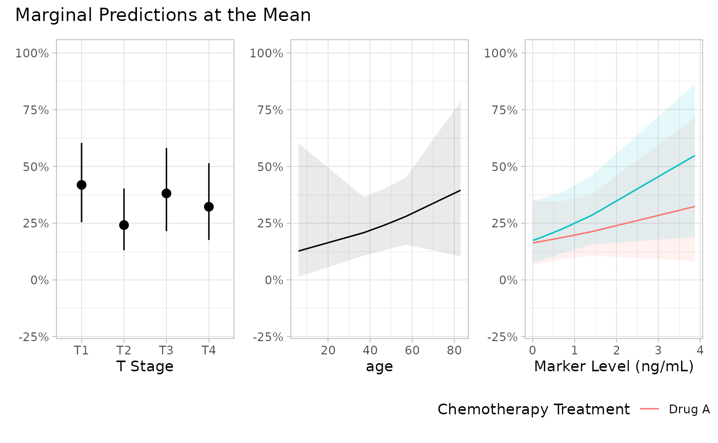
p <- mod |>
  plot_marginal_predictions(newdata = "mean") |>
  patchwork::wrap_plots() &
  ggplot2::scale_y_continuous(
    labels = scales::label_percent(),
    limits = c(-0.2, 1)
  )
p[[2]] <- p[[2]] + ggplot2::xlab("Age in years")
p + patchwork::plot_annotation(
  title = "Marginal Predictions at the Mean"
)

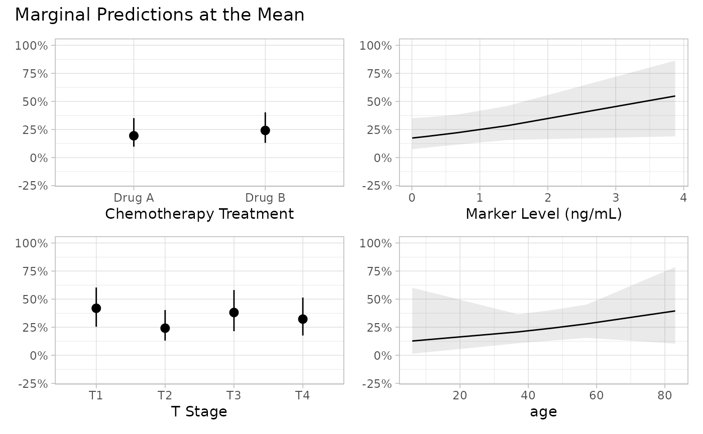
p <- mod |>
  plot_marginal_predictions(
    "no_interaction",
    newdata = "mean"
  ) |>
  patchwork::wrap_plots() &
  ggplot2::scale_y_continuous(
    labels = scales::label_percent(),
    limits = c(-0.2, 1)
  )
p[[4]] <- p[[4]] + ggplot2::xlab("Age in years")
p + patchwork::plot_annotation(
  title = "Marginal Predictions at the Mean"
)

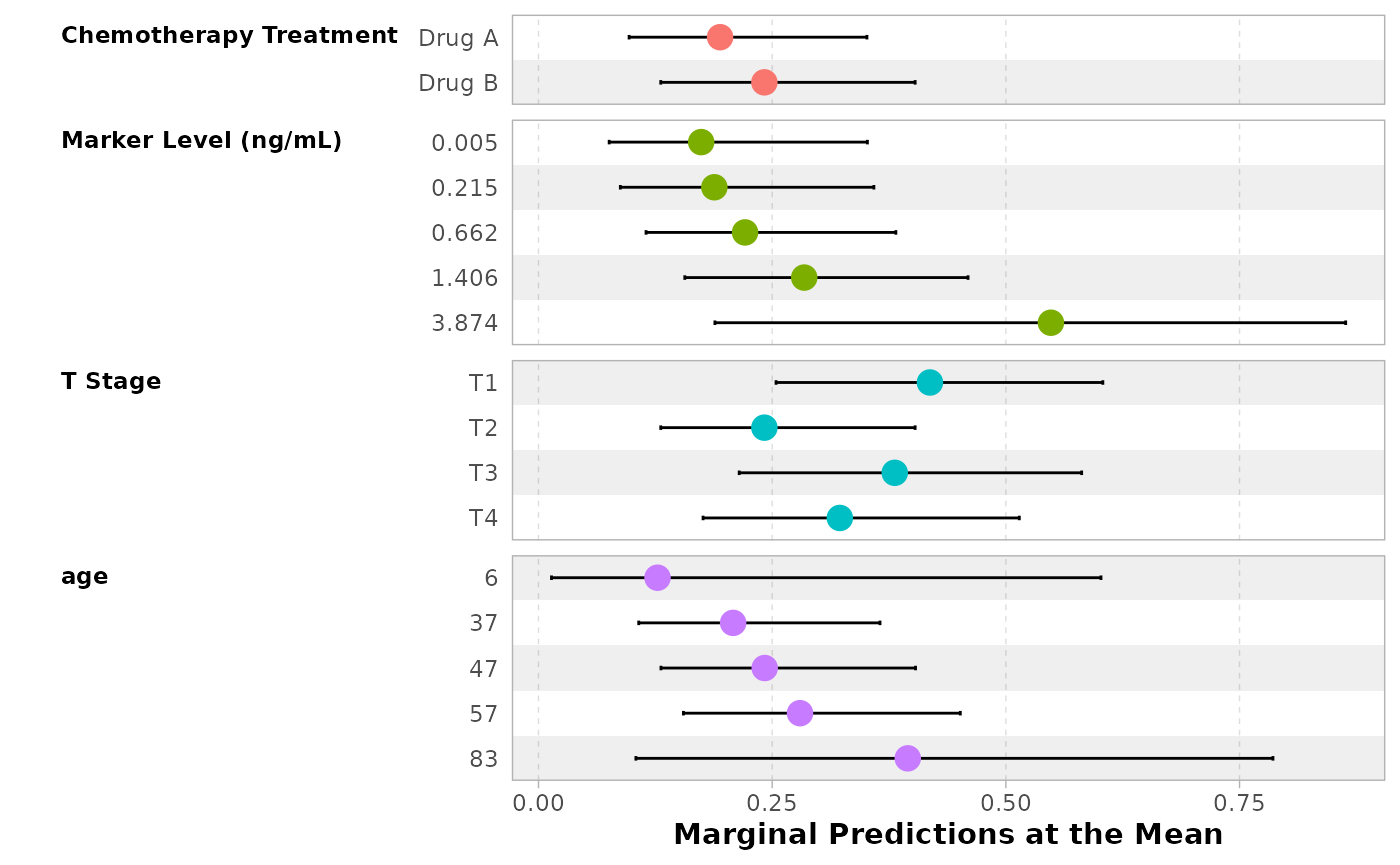
Alternatively, you can use ggstats::ggcoef_model(), using tidy_args to pass arguments to broom.helpers::tidy_marginal_predictions().

ggstats::ggcoef_model(
  mod,
  tidy_fun = tidy_marginal_predictions,
  tidy_args = list(newdata = "mean", variables_list = "no_interaction"),
  vline = FALSE,
  show_p_values = FALSE,
  signif_stars = FALSE,
  significance = NULL,
  variable_labels = c(age = "Age in years")
)

Average Marginal Predictions

Instead of averaging observed values to generate “typical observations” before predicting the outcome, an alternative consists to predict the outcome on the overall observed values before averaging the results.

More precisely, the purpose is to adopt a counterfactual approach. Let’s take an example. Let’s consider d our observed data used to estimate the model. We can make a copy of this dataset, where all variables would be identical, but considering that all individuals have received Drug A. Similarly, we could generate a dataset where all individuals would have received Drug B.

dA <- d |>
  mutate(trt = "Drug A")
dB <- d |>
  mutate(trt = "Drug B")

We can now predict the outcome for all observations in dA and then compute the average, and similarly with dB.

predict(mod, newdata = dA, type = "response") |> mean()
#> [1] 0.2830866
predict(mod, newdata = dB, type = "response") |> mean()
#> [1] 0.3431492

We, then, obtain Average Marginal Predictions for trt. The same results could be computed with marginaleffects::avg_predictions(). Note that the counterfactual approach corresponds to the default behavior when no value is provided to newdata.

avg_predictions(mod, variables = "trt", by = "trt", type = "response")
#> 
#>     trt Estimate Std. Error    z Pr(>|z|)    S 2.5 % 97.5 %
#>  Drug A    0.283     0.0484 5.85   <0.001 27.6 0.188  0.378
#>  Drug B    0.343     0.0490 7.01   <0.001 38.6 0.247  0.439
#> 
#> Columns: trt, estimate, std.error, statistic, p.value, s.value, conf.low, conf.high 
#> Type:  response

Important: since version 0.10.0 of marginaleffects, we had to add type = "response" to get this result: for glm models, predictions are done on the response scale, before being averaged. If type are not specified, predictions will be made on the link scale, before being averaged and then back transformed on the response scale. Thus, the average prediction may not be exactly identical to the average of predictions.

avg_predictions(mod, variables = "trt", by = "trt")
#> 
#>     trt Estimate Pr(>|z|)    S 2.5 % 97.5 %
#>  Drug A    0.274  < 0.001 13.1 0.187  0.383
#>  Drug B    0.333  0.00279  8.5 0.241  0.441
#> 
#> Columns: trt, estimate, p.value, s.value, conf.low, conf.high 
#> Type:  invlink(link)
b <- binomial()
predict(mod, newdata = dA, type = "link") |>
  mean() |>
  b$linkinv()
#> [1] 0.2743123
predict(mod, newdata = dB, type = "link") |>
  mean() |>
  b$linkinv()
#> [1] 0.3331447

We can use tidy_marginal_predictions() to get average marginal predictions for all variables and plot_marginal_predictions() for a visual representation.

mod |>
  tbl_regression(
    tidy_fun = tidy_marginal_predictions,
    type = "response",
    variables_list = "no_interaction",
    estimate_fun = scales::label_percent(accuracy = .1),
    label = list(age = "Age in years")
  ) |>
  modify_column_hide("p.value") |>
  bold_labels()

Characteristic	Average Marginal Predictions	95% CI¹
Chemotherapy Treatment
Drug A	28.3%	18.8%, 37.8%
Drug B	34.3%	24.7%, 43.9%
Marker Level (ng/mL)
0.005	25.0%	15.9%, 34.0%
0.215	26.3%	18.0%, 34.6%
0.662	29.3%	22.3%, 36.4%
1.406	34.8%	26.8%, 42.8%
3.874	54.5%	28.5%, 80.4%
T Stage
T1	38.9%	24.9%, 52.9%
T2	22.5%	11.2%, 33.8%
T3	35.4%	20.0%, 50.8%
T4	30.0%	16.1%, 43.8%
Age in years
6	17.4%	-12.9%, 47.6%
37	27.1%	18.8%, 35.4%
47	30.9%	22.4%, 39.5%
57	35.1%	26.0%, 44.2%
83	47.1%	10.0%, 84.2%
¹ CI = Confidence Interval

mod |>
  tbl_regression(
    tidy_fun = tidy_marginal_predictions,
    type = "response",
    estimate_fun = scales::label_percent(accuracy = .1),
    label = list(age = "Age in years")
  ) |>
  modify_column_hide("p.value") |>
  bold_labels()

Characteristic	Average Marginal Predictions	95% CI¹
T Stage
T1	38.9%	24.9%, 52.9%
T2	22.5%	11.2%, 33.8%
T3	35.4%	20.0%, 50.8%
T4	30.0%	16.1%, 43.8%
Age in years
6	17.4%	-12.9%, 47.6%
37	27.1%	18.8%, 35.4%
47	30.9%	22.4%, 39.5%
57	35.1%	26.0%, 44.2%
83	47.1%	10.0%, 84.2%
Chemotherapy Treatment * Marker Level (ng/mL)
Drug A * 0.005	24.2%	10.9%, 37.6%
Drug A * 0.215	25.1%	13.0%, 37.3%
Drug A * 0.662	27.0%	16.9%, 37.2%
Drug A * 1.406	30.5%	19.9%, 41.0%
Drug A * 3.874	43.1%	5.7%, 80.5%
Drug B * 0.005	25.6%	13.4%, 37.9%
Drug B * 0.215	27.4%	16.2%, 38.7%
Drug B * 0.662	31.5%	21.6%, 41.3%
Drug B * 1.406	38.8%	26.9%, 50.7%
Drug B * 3.874	64.9%	29.3%, 100.6%
¹ CI = Confidence Interval

p <- plot_marginal_predictions(mod, type = "response") |>
  patchwork::wrap_plots(ncol = 2) &
  ggplot2::scale_y_continuous(
    labels = scales::label_percent(),
    limits = c(-0.2, 1)
  )
p[[2]] <- p[[2]] + ggplot2::xlab("Age in years")
p + patchwork::plot_annotation(
  title = "Average Marginal Predictions"
)

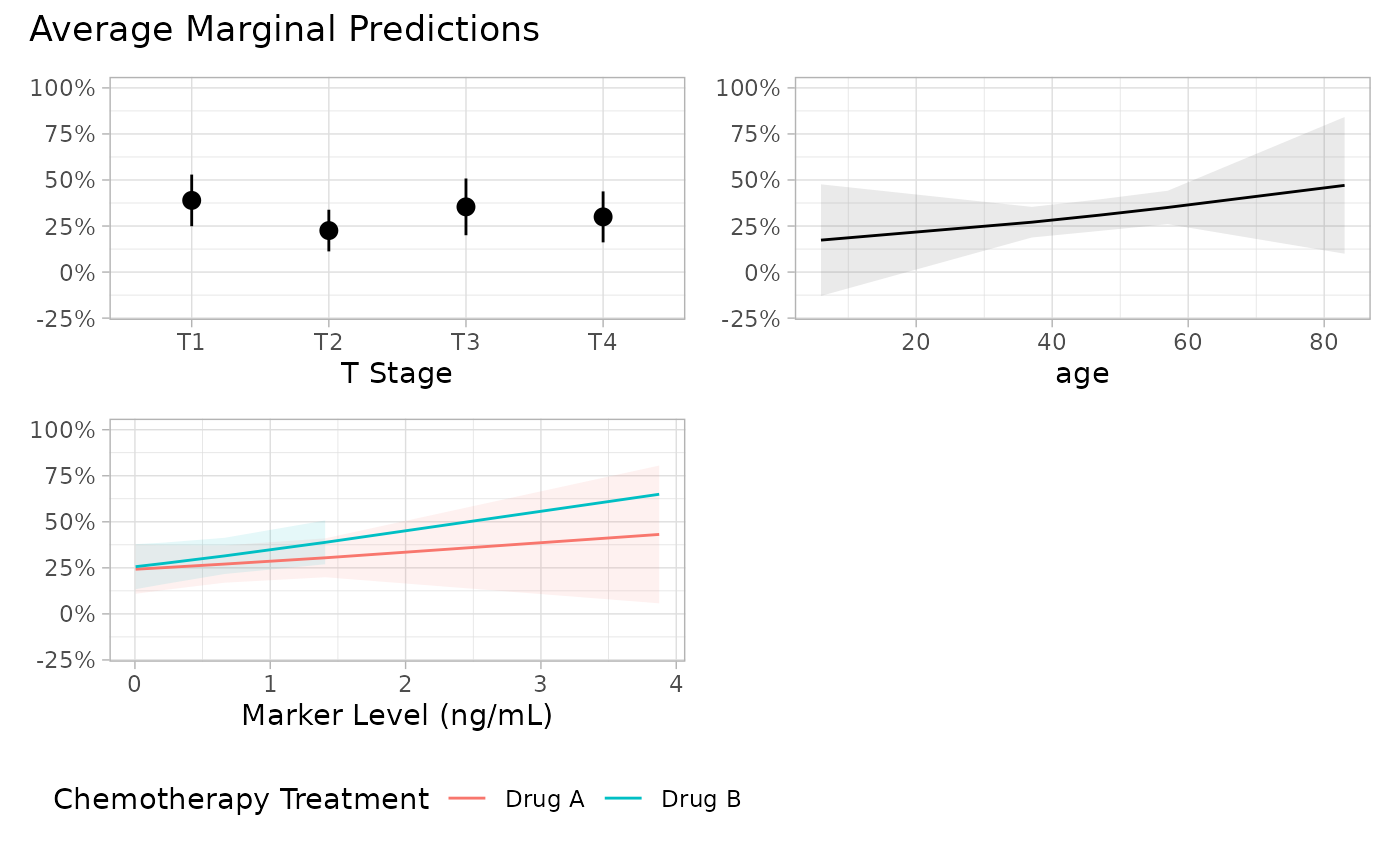
Marginal Means and Marginal Predictions at Marginal Means

The emmeans package adopted, by default, another approach based on marginal means or estimated marginal means (a.k.a. emmeans).

It will consider a grid of predictors with all combinations of the observed modalities of the categorical variables and fixing continuous variables at their means.

Let’s call marginaleffects::predictions() with newdata = "marginalmeans".

pred <- predictions(mod, newdata = "marginalmeans")
pred
#> 
#>  Estimate Pr(>|z|)    S  2.5 % 97.5 %
#>     0.353  0.11462  3.1 0.2042  0.537
#>     0.194  < 0.001 10.8 0.0969  0.351
#>     0.318  0.07405  3.8 0.1678  0.519
#>     0.265  0.01648  5.9 0.1351  0.453
#>     0.419  0.39097  1.4 0.2541  0.604
#>     0.242  0.00282  8.5 0.1308  0.403
#>     0.381  0.24194  2.0 0.2147  0.581
#>     0.322  0.06889  3.9 0.1760  0.514
#> 
#> Columns: rowid, estimate, p.value, s.value, conf.low, conf.high, trt, marker, stage, age, response 
#> Type:  invlink(link)

As we can see, pred contains 8 rows, one for each combination of trt (2 modalities) and stage (4 modalities). age is fixed at its mean (mean(d$age)) as well as marker.

Let’s compute the average predictions for each value of stage.

pred |>
  group_by(stage) |>
  summarise(mean(estimate))
#> # A tibble: 4 × 2
#>   stage `mean(estimate)`
#>   <fct>            <dbl>
#> 1 T1               0.386
#> 2 T2               0.218
#> 3 T3               0.349
#> 4 T4               0.294

We can check that we obtain the same estimates as with emmeans::emmeans().

emmeans::emmeans(mod, "stage", type = "response")
#>  stage  prob     SE  df asymp.LCL asymp.UCL
#>  T1    0.385 0.0813 Inf     0.242     0.551
#>  T2    0.217 0.0611 Inf     0.120     0.359
#>  T3    0.349 0.0874 Inf     0.201     0.532
#>  T4    0.293 0.0788 Inf     0.164     0.466
#> 
#> Results are averaged over the levels of: trt 
#> Confidence level used: 0.95 
#> Intervals are back-transformed from the logit scale

These estimates could be computed, for each categorical variable, with marginaleffects::prediction() using datagrid(grid_type = "balanced")¹.

predictions(mod,
  by = "trt",
  newdata = datagrid(grid_type = "balanced")
)
#> 
#>     trt Estimate Pr(>|z|)    S 2.5 % 97.5 %
#>  Drug A    0.278   <0.001 10.1 0.180  0.403
#>  Drug B    0.337   0.0104  6.6 0.233  0.460
#> 
#> Columns: trt, estimate, p.value, s.value, conf.low, conf.high 
#> Type:  invlink(link)
predictions(mod,
  by = "stage",
  newdata = datagrid(grid_type = "balanced")
)
#> 
#>  stage Estimate Pr(>|z|)    S 2.5 % 97.5 %
#>     T1    0.385   0.1734  2.5 0.242  0.551
#>     T2    0.217   <0.001 11.4 0.120  0.359
#>     T3    0.349   0.1047  3.3 0.201  0.532
#>     T4    0.293   0.0205  5.6 0.164  0.466
#> 
#> Columns: stage, estimate, p.value, s.value, conf.low, conf.high 
#> Type:  invlink(link)

Marginal means are defined only for categorical variables. However, we can define marginal predictions at marginal means for both continuous and categorical variables, calling tidy_marginal_predictions() with the option newdata = "marginalmeans". For categorical variables, marginal predictions at marginal means will be equal to marginal means.

mod |>
  tbl_regression(
    tidy_fun = tidy_marginal_predictions,
    newdata = "marginalmeans",
    variables_list = "no_interaction",
    estimate_fun = scales::label_percent(accuracy = .1),
    label = list(age = "Age in years")
  ) |>
  modify_column_hide("p.value") |>
  bold_labels()

Characteristic	Marginal Predictions at Marginal Means	95% CI¹
Chemotherapy Treatment
Drug A	27.8%	18.0%, 40.3%
Drug B	33.7%	23.3%, 46.0%
Marker Level (ng/mL)
0.005	24.5%	15.3%, 36.8%
0.215	25.8%	17.0%, 37.2%
0.662	28.9%	20.6%, 38.8%
1.406	34.4%	25.2%, 44.8%
3.874	54.9%	27.9%, 79.3%
T Stage
T1	38.5%	24.2%, 55.1%
T2	21.7%	12.0%, 35.9%
T3	34.9%	20.1%, 53.2%
T4	29.3%	16.4%, 46.6%
Age in years
6	16.9%	2.3%, 64.0%
37	26.8%	19.0%, 36.3%
47	30.7%	22.5%, 40.4%
57	35.1%	26.2%, 45.1%
83	47.6%	16.1%, 81.1%
¹ CI = Confidence Interval

Alternative approaches

Marginal Predictions at the Median

They are similar to marginal predictions at the mean, except that continuous variables are fixed at the median of observed values (and categorical variables at their mode). Simply use newdata = "median".

mod |>
  tbl_regression(
    tidy_fun = tidy_marginal_predictions,
    newdata = "median",
    variables_list = "no_interaction",
    estimate_fun = scales::label_percent(accuracy = .1),
    label = list(age = "Age in years")
  ) |>
  modify_column_hide("p.value") |>
  bold_labels()

Characteristic	Marginal Predictions	95% CI¹
Chemotherapy Treatment
Drug A	18.5%	8.9%, 34.6%
Drug B	22.1%	11.5%, 38.3%
Marker Level (ng/mL)
0.005	17.4%	7.6%, 35.2%
0.215	18.8%	8.8%, 35.9%
0.662	22.1%	11.5%, 38.3%
1.406	28.5%	15.7%, 46.0%
3.874	54.9%	18.9%, 86.4%
T Stage
T1	39.1%	23.2%, 57.7%
T2	22.1%	11.5%, 38.3%
T3	35.5%	19.3%, 55.7%
T4	29.8%	16.0%, 48.7%
Age in years
6	11.5%	1.2%, 57.6%
37	19.0%	9.4%, 34.6%
47	22.1%	11.5%, 38.3%
57	25.7%	13.7%, 42.9%
83	36.8%	9.3%, 76.6%
¹ CI = Confidence Interval

the `ggeffects::ggpredict()`’s approach

The ggeffects package offers a ggeffects::ggpredict() function which generates marginal predictions at the mean of continuous variables and at the first modality (used as reference) of categorical variables. broom.helpers provides a tidy_ggpredict() tidier.

mod |>
  tbl_regression(
    tidy_fun = tidy_ggpredict,
    estimate_fun = scales::label_percent(accuracy = .1),
    label = list(age = "Age in years")
  ) |>
  bold_labels()
#> Warning: Some of the focal terms are of type `character`. This may lead to
#>   unexpected results. It is recommended to convert these variables to
#>   factors before fitting the model.
#>   The following variables in are of type character: `trt`

Characteristic	Marginal Predictions	95% CI¹
Chemotherapy Treatment
Drug A	35.3%	20.4%, 53.7%
Drug B	41.9%	25.4%, 60.4%
Marker Level (ng/mL)
0.005	32.3%	16.7%, 53.1%
0.013	32.3%	16.8%, 53.2%
0.015	32.4%	16.8%, 53.2%
0.021	32.4%	16.8%, 53.2%
0.022	32.4%	16.9%, 53.2%
0.039	32.6%	17.0%, 53.3%
0.043	32.6%	17.1%, 53.3%
0.045	32.7%	17.1%, 53.3%
0.046	32.7%	17.1%, 53.3%
0.056	32.8%	17.2%, 53.4%
0.06	32.8%	17.2%, 53.4%
0.062	32.8%	17.3%, 53.4%
0.063	32.8%	17.3%, 53.4%
0.066	32.9%	17.3%, 53.4%
0.075	33.0%	17.4%, 53.5%
0.081	33.0%	17.5%, 53.5%
0.086	33.1%	17.5%, 53.5%
0.092	33.1%	17.6%, 53.5%
0.096	33.2%	17.6%, 53.6%
0.105	33.3%	17.7%, 53.6%
0.108	33.3%	17.7%, 53.6%
0.124	33.5%	17.9%, 53.7%
0.128	33.5%	17.9%, 53.7%
0.131	33.5%	18.0%, 53.7%
0.136	33.6%	18.0%, 53.8%
0.141	33.6%	18.1%, 53.8%
0.144	33.7%	18.1%, 53.8%
0.153	33.7%	18.2%, 53.9%
0.157	33.8%	18.2%, 53.9%
0.16	33.8%	18.3%, 53.9%
0.161	33.8%	18.3%, 53.9%
0.169	33.9%	18.3%, 54.0%
0.175	34.0%	18.4%, 54.0%
0.177	34.0%	18.4%, 54.0%
0.182	34.0%	18.5%, 54.0%
0.205	34.3%	18.7%, 54.2%
0.215	34.4%	18.8%, 54.2%
0.22	34.4%	18.9%, 54.3%
0.222	34.5%	18.9%, 54.3%
0.229	34.5%	19.0%, 54.3%
0.238	34.6%	19.0%, 54.4%
0.239	34.6%	19.1%, 54.4%
0.243	34.7%	19.1%, 54.4%
0.25	34.7%	19.2%, 54.4%
0.258	34.8%	19.3%, 54.5%
0.266	34.9%	19.3%, 54.5%
0.277	35.0%	19.4%, 54.6%
0.29	35.1%	19.6%, 54.7%
0.305	35.3%	19.7%, 54.8%
0.308	35.3%	19.8%, 54.8%
0.309	35.3%	19.8%, 54.8%
0.325	35.5%	19.9%, 54.9%
0.333	35.6%	20.0%, 55.0%
0.352	35.8%	20.2%, 55.1%
0.354	35.8%	20.2%, 55.1%
0.358	35.9%	20.3%, 55.1%
0.361	35.9%	20.3%, 55.2%
0.37	36.0%	20.4%, 55.2%
0.385	36.1%	20.5%, 55.3%
0.386	36.1%	20.5%, 55.3%
0.387	36.2%	20.6%, 55.4%
0.389	36.2%	20.6%, 55.4%
0.402	36.3%	20.7%, 55.5%
0.408	36.4%	20.8%, 55.5%
0.445	36.8%	21.1%, 55.8%
0.475	37.1%	21.4%, 56.0%
0.51	37.5%	21.8%, 56.3%
0.511	37.5%	21.8%, 56.3%
0.513	37.5%	21.8%, 56.3%
0.531	37.7%	22.0%, 56.5%
0.547	37.8%	22.1%, 56.6%
0.583	38.2%	22.5%, 56.9%
0.589	38.3%	22.5%, 57.0%
0.592	38.3%	22.6%, 57.0%
0.599	38.4%	22.6%, 57.1%
0.611	38.5%	22.7%, 57.2%
0.613	38.5%	22.8%, 57.2%
0.615	38.6%	22.8%, 57.2%
0.662	39.1%	23.2%, 57.7%
0.667	39.1%	23.3%, 57.7%
0.691	39.4%	23.5%, 57.9%
0.702	39.5%	23.6%, 58.0%
0.711	39.6%	23.7%, 58.1%
0.717	39.7%	23.7%, 58.2%
0.718	39.7%	23.7%, 58.2%
0.719	39.7%	23.7%, 58.2%
0.733	39.8%	23.8%, 58.3%
0.737	39.9%	23.9%, 58.4%
0.772	40.3%	24.2%, 58.7%
0.803	40.6%	24.5%, 59.1%
0.816	40.7%	24.6%, 59.2%
0.831	40.9%	24.7%, 59.4%
0.862	41.2%	25.0%, 59.7%
0.895	41.6%	25.2%, 60.1%
0.924	41.9%	25.5%, 60.4%
0.929	42.0%	25.5%, 60.5%
0.946	42.2%	25.6%, 60.7%
0.976	42.5%	25.9%, 61.0%
0.981	42.6%	25.9%, 61.1%
1.041	43.2%	26.3%, 61.8%
1.046	43.3%	26.4%, 61.9%
1.061	43.4%	26.5%, 62.1%
1.063	43.5%	26.5%, 62.1%
1.075	43.6%	26.6%, 62.3%
1.079	43.6%	26.6%, 62.3%
1.087	43.7%	26.7%, 62.4%
1.091	43.8%	26.7%, 62.5%
1.107	44.0%	26.8%, 62.7%
1.129	44.2%	27.0%, 63.0%
1.133	44.3%	27.0%, 63.0%
1.148	44.4%	27.1%, 63.2%
1.156	44.5%	27.1%, 63.3%
1.2	45.0%	27.4%, 63.9%
1.206	45.1%	27.5%, 64.0%
1.207	45.1%	27.5%, 64.0%
1.225	45.3%	27.6%, 64.3%
1.255	45.6%	27.8%, 64.7%
1.306	46.2%	28.0%, 65.4%
1.321	46.4%	28.1%, 65.6%
1.354	46.7%	28.3%, 66.1%
1.406	47.3%	28.6%, 66.8%
1.418	47.5%	28.6%, 67.0%
1.441	47.7%	28.8%, 67.3%
1.479	48.1%	28.9%, 67.9%
1.491	48.3%	29.0%, 68.1%
1.527	48.7%	29.2%, 68.6%
1.55	48.9%	29.3%, 68.9%
1.628	49.8%	29.6%, 70.1%
1.645	50.0%	29.7%, 70.4%
1.658	50.2%	29.7%, 70.6%
1.68	50.4%	29.8%, 70.9%
1.709	50.7%	29.9%, 71.3%
1.713	50.8%	29.9%, 71.4%
1.739	51.1%	30.0%, 71.8%
1.804	51.8%	30.2%, 72.8%
1.869	52.5%	30.4%, 73.7%
1.882	52.7%	30.4%, 73.9%
1.892	52.8%	30.5%, 74.1%
1.894	52.8%	30.5%, 74.1%
1.941	53.4%	30.6%, 74.8%
1.976	53.8%	30.7%, 75.3%
1.985	53.9%	30.7%, 75.4%
2.008	54.1%	30.8%, 75.8%
2.032	54.4%	30.8%, 76.1%
2.083	55.0%	30.9%, 76.9%
2.124	55.4%	31.0%, 77.5%
2.141	55.6%	31.1%, 77.7%
2.19	56.2%	31.1%, 78.4%
2.213	56.4%	31.2%, 78.7%
2.238	56.7%	31.2%, 79.0%
2.288	57.2%	31.3%, 79.7%
2.345	57.9%	31.4%, 80.5%
2.447	59.0%	31.5%, 81.8%
2.522	59.8%	31.6%, 82.8%
2.636	61.0%	31.7%, 84.1%
2.702	61.8%	31.7%, 84.9%
2.725	62.0%	31.7%, 85.1%
2.767	62.4%	31.7%, 85.6%
3.02	65.1%	31.8%, 88.2%
3.062	65.5%	31.8%, 88.6%
3.249	67.4%	31.8%, 90.2%
3.642	71.2%	31.7%, 92.9%
3.751	72.2%	31.6%, 93.6%
3.874	73.3%	31.5%, 94.2%
T Stage
T1	41.9%	25.4%, 60.4%
T2	24.2%	13.1%, 40.3%
T3	38.1%	21.5%, 58.1%
T4	32.2%	17.6%, 51.4%
Age in years
6	24.8%	3.4%, 75.6%
9	25.9%	4.7%, 71.2%
10	26.2%	5.2%, 69.8%
17	28.9%	9.5%, 60.9%
19	29.6%	11.0%, 59.0%
20	30.0%	11.7%, 58.1%
21	30.4%	12.5%, 57.3%
23	31.3%	14.0%, 56.0%
25	32.1%	15.4%, 55.0%
26	32.5%	16.1%, 54.6%
27	32.9%	16.8%, 54.4%
28	33.3%	17.4%, 54.2%
30	34.2%	18.6%, 54.1%
31	34.6%	19.2%, 54.2%
32	35.1%	19.7%, 54.3%
34	35.9%	20.7%, 54.7%
35	36.4%	21.1%, 55.0%
36	36.8%	21.5%, 55.4%
37	37.3%	21.9%, 55.7%
38	37.7%	22.3%, 56.2%
39	38.2%	22.7%, 56.6%
40	38.7%	23.0%, 57.1%
41	39.1%	23.4%, 57.5%
42	39.6%	23.7%, 58.0%
43	40.0%	24.0%, 58.5%
44	40.5%	24.4%, 59.0%
45	41.0%	24.7%, 59.5%
46	41.5%	25.1%, 59.9%
47	41.9%	25.4%, 60.4%
48	42.4%	25.8%, 60.9%
49	42.9%	26.2%, 61.4%
50	43.4%	26.6%, 61.8%
51	43.8%	26.9%, 62.3%
52	44.3%	27.3%, 62.8%
53	44.8%	27.7%, 63.2%
54	45.3%	28.1%, 63.7%
55	45.8%	28.5%, 64.1%
56	46.3%	28.9%, 64.6%
57	46.8%	29.2%, 65.1%
58	47.3%	29.6%, 65.6%
59	47.7%	29.9%, 66.2%
60	48.2%	30.2%, 66.7%
61	48.7%	30.5%, 67.3%
62	49.2%	30.7%, 67.9%
63	49.7%	30.9%, 68.6%
64	50.2%	31.1%, 69.3%
65	50.7%	31.2%, 70.1%
66	51.2%	31.2%, 70.9%
67	51.7%	31.2%, 71.7%
68	52.2%	31.0%, 72.6%
69	52.7%	30.9%, 73.6%
70	53.2%	30.6%, 74.6%
71	53.7%	30.3%, 75.6%
74	55.2%	28.9%, 78.9%
75	55.7%	28.3%, 80.0%
76	56.2%	27.6%, 81.2%
78	57.2%	26.1%, 83.4%
83	59.6%	21.6%, 88.8%
¹ CI = Confidence Interval

mod |>
  ggeffects::ggpredict() |>
  plot() |>
  patchwork::wrap_plots()
#> Warning: Some of the focal terms are of type `character`. This may lead to
#>   unexpected results. It is recommended to convert these variables to
#>   factors before fitting the model.
#>   The following variables in are of type character: `trt`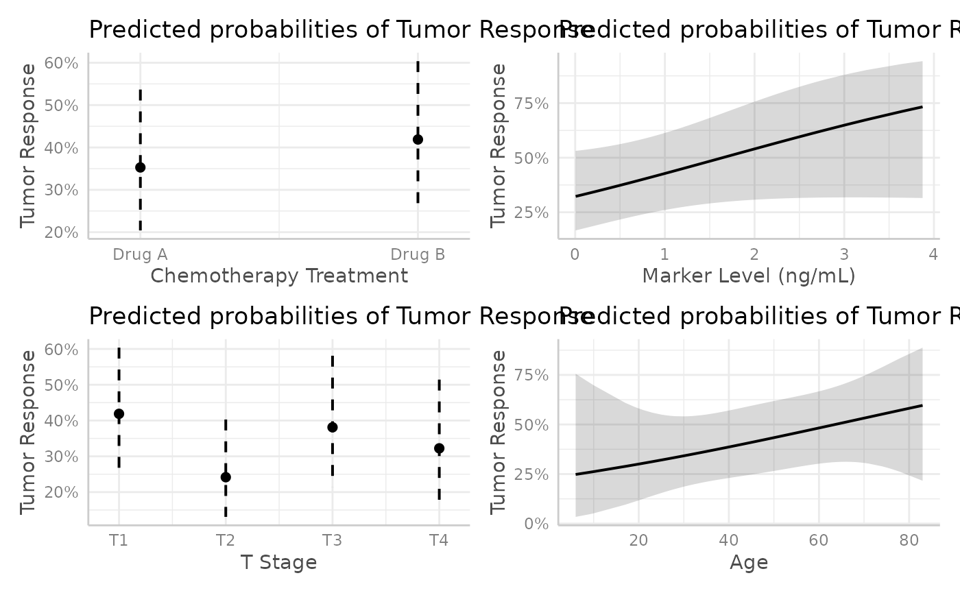

Marginal Contrasts

Now that we have a way to estimate marginal predictions, we can easily compute marginal contrasts, i.e. difference between marginal predictions.

Average Marginal Contrasts

Let’s consider first a categorical variable, e.g. stage. Average Marginal Predictions are obtained with marginaleffects::avg_predictions().

pred <- avg_predictions(mod, variables = "stage", by = "stage", type = "response")
pred
#> 
#>  stage Estimate Std. Error    z Pr(>|z|)    S 2.5 % 97.5 %
#>     T1    0.389     0.0715 5.44   <0.001 24.2 0.249  0.529
#>     T2    0.225     0.0577 3.91   <0.001 13.4 0.112  0.338
#>     T4    0.300     0.0706 4.25   <0.001 15.5 0.161  0.438
#>     T3    0.354     0.0786 4.51   <0.001 17.2 0.200  0.508
#> 
#> Columns: stage, estimate, std.error, statistic, p.value, s.value, conf.low, conf.high 
#> Type:  response

The contrast between "T2" and "T1" is simply the difference between the two adjusted predictions:

pred$estimate[2] - pred$estimate[1]
#> [1] -0.1637819

The marginaleffects::avg_comparisons() function allows to compute all differences between adjusted predictions.

comp <- avg_comparisons(mod, variables = "stage")
comp
#> 
#>   Term            Contrast Estimate Std. Error      z Pr(>|z|)   S  2.5 %
#>  stage mean(T2) - mean(T1)  -0.1638     0.0925 -1.770   0.0767 3.7 -0.345
#>  stage mean(T3) - mean(T1)  -0.0351     0.1065 -0.330   0.7417 0.4 -0.244
#>  stage mean(T4) - mean(T1)  -0.0895     0.1004 -0.891   0.3727 1.4 -0.286
#>  97.5 %
#>  0.0175
#>  0.1736
#>  0.1073
#> 
#> Columns: term, contrast, estimate, std.error, statistic, p.value, s.value, conf.low, conf.high, predicted_lo, predicted_hi, predicted 
#> Type:  response

Note: in fact, avg_comparisons() has computed the contrasts for each observed values before averaging it. By construction, it is equivalent to the difference of the average marginal predictions.

As the contrast has been averaged over the observed values, we can call them average marginal contrast.

By default, each modality is contrasted with the first one taken as a reference.

avg_comparisons(mod, variables = "stage")
#> 
#>   Term            Contrast Estimate Std. Error      z Pr(>|z|)   S  2.5 %
#>  stage mean(T2) - mean(T1)  -0.1638     0.0925 -1.770   0.0767 3.7 -0.345
#>  stage mean(T3) - mean(T1)  -0.0351     0.1065 -0.330   0.7417 0.4 -0.244
#>  stage mean(T4) - mean(T1)  -0.0895     0.1004 -0.891   0.3727 1.4 -0.286
#>  97.5 %
#>  0.0175
#>  0.1736
#>  0.1073
#> 
#> Columns: term, contrast, estimate, std.error, statistic, p.value, s.value, conf.low, conf.high, predicted_lo, predicted_hi, predicted 
#> Type:  response

Other types of contrasts could be specified using the variables argument.

avg_comparisons(mod, variables = list(stage = "sequential"))
#> 
#>   Term            Contrast Estimate Std. Error      z Pr(>|z|)   S   2.5 %
#>  stage mean(T2) - mean(T1)  -0.1638     0.0925 -1.770   0.0767 3.7 -0.3451
#>  stage mean(T3) - mean(T2)   0.1287     0.0972  1.324   0.1856 2.4 -0.0619
#>  stage mean(T4) - mean(T3)  -0.0544     0.1060 -0.513   0.6081 0.7 -0.2622
#>  97.5 %
#>  0.0175
#>  0.3192
#>  0.1535
#> 
#> Columns: term, contrast, estimate, std.error, statistic, p.value, s.value, conf.low, conf.high, predicted_lo, predicted_hi, predicted 
#> Type:  response
avg_comparisons(mod, variables = list(stage = "pairwise"))
#> 
#>   Term            Contrast Estimate Std. Error      z Pr(>|z|)   S   2.5 %
#>  stage mean(T2) - mean(T1)  -0.1638     0.0925 -1.770   0.0767 3.7 -0.3451
#>  stage mean(T3) - mean(T1)  -0.0351     0.1065 -0.330   0.7417 0.4 -0.2437
#>  stage mean(T3) - mean(T2)   0.1287     0.0972  1.324   0.1856 2.4 -0.0619
#>  stage mean(T4) - mean(T1)  -0.0895     0.1004 -0.891   0.3727 1.4 -0.2862
#>  stage mean(T4) - mean(T2)   0.0743     0.0917  0.811   0.4176 1.3 -0.1054
#>  stage mean(T4) - mean(T3)  -0.0544     0.1060 -0.513   0.6081 0.7 -0.2622
#>  97.5 %
#>  0.0175
#>  0.1736
#>  0.3192
#>  0.1073
#>  0.2540
#>  0.1535
#> 
#> Columns: term, contrast, estimate, std.error, statistic, p.value, s.value, conf.low, conf.high, predicted_lo, predicted_hi, predicted 
#> Type:  response

Let’s consider a continuous variable:

avg_comparisons(mod, variables = "age")
#> 
#>  Term Contrast Estimate Std. Error    z Pr(>|z|)   S  2.5 %  97.5 %
#>   age mean(+1)  0.00399    0.00239 1.67   0.0954 3.4 -7e-04 0.00868
#> 
#> Columns: term, contrast, estimate, std.error, statistic, p.value, s.value, conf.low, conf.high, predicted_lo, predicted_hi, predicted 
#> Type:  response

By default, marginaleffects::avg_comparisons() computes, for each observed value, the effect of increasing age by one unit (comparing adjusted predictions when the regressor is equal to its observed value minus 0.5 and its observed value plus 0.5). It is possible to compute a contrast for another gap, for example the average difference for an increase of 10 years:

avg_comparisons(mod, variables = list(age = 10))
#> 
#>  Term  Contrast Estimate Std. Error    z Pr(>|z|)   S   2.5 % 97.5 %
#>   age mean(+10)   0.0412     0.0288 1.43    0.152 2.7 -0.0152 0.0976
#> 
#> Columns: term, contrast, estimate, std.error, statistic, p.value, s.value, conf.low, conf.high, predicted_lo, predicted_hi, predicted 
#> Type:  response

Contrasts for all individual predictors could be easily obtained:

avg_comparisons(mod)
#> 
#>    Term                    Contrast Estimate Std. Error      z Pr(>|z|)   S
#>  age    mean(+1)                     0.00399    0.00239  1.667   0.0954 3.4
#>  marker mean(+1)                     0.07470    0.04150  1.800   0.0719 3.8
#>  stage  mean(T2) - mean(T1)         -0.16378    0.09252 -1.770   0.0767 3.7
#>  stage  mean(T3) - mean(T1)         -0.03509    0.10646 -0.330   0.7417 0.4
#>  stage  mean(T4) - mean(T1)         -0.08947    0.10037 -0.891   0.3727 1.4
#>  trt    mean(Drug B) - mean(Drug A)  0.06006    0.06893  0.871   0.3836 1.4
#>     2.5 %  97.5 %
#>  -0.00070 0.00868
#>  -0.00664 0.15604
#>  -0.34511 0.01755
#>  -0.24374 0.17356
#>  -0.28620 0.10726
#>  -0.07504 0.19517
#> 
#> Columns: term, contrast, estimate, std.error, statistic, p.value, s.value, conf.low, conf.high, predicted_lo, predicted_hi, predicted 
#> Type:  response

It should be noted that column names are not consistent with other tidiers used by broom.helpers. Therefore, a comparisons object should not be passed directly to tidy_plus_plus(). Instead, you should use broom.helpers::tidy_avg_comparisons().

tidy_avg_comparisons(mod)
#> # A tibble: 6 × 12
#>   variable term  estimate std.error statistic p.value s.value conf.low conf.high
#>   <chr>    <chr>    <dbl>     <dbl>     <dbl>   <dbl>   <dbl>    <dbl>     <dbl>
#> 1 age      mean…  0.00399   0.00239     1.67   0.0954   3.39  -7.00e-4   0.00868
#> 2 marker   mean…  0.0747    0.0415      1.80   0.0719   3.80  -6.64e-3   0.156  
#> 3 stage    mean… -0.164     0.0925     -1.77   0.0767   3.71  -3.45e-1   0.0175 
#> 4 stage    mean… -0.0351    0.106      -0.330  0.742    0.431 -2.44e-1   0.174  
#> 5 stage    mean… -0.0895    0.100      -0.891  0.373    1.42  -2.86e-1   0.107  
#> 6 trt      mean…  0.0601    0.0689      0.871  0.384    1.38  -7.50e-2   0.195  
#> # ℹ 3 more variables: predicted_lo <dbl>, predicted_hi <dbl>, predicted <dbl>

This custom tidier is compatible with tidy_plus_plus() and the suit of other functions provided by broom.helpers.

mod |>
  tidy_plus_plus(tidy_fun = tidy_avg_comparisons)
#> # A tibble: 6 × 23
#>   term               variable var_label var_class var_type var_nlevels contrasts
#>   <chr>              <chr>    <chr>     <chr>     <chr>          <int> <chr>    
#> 1 mean(+1)           age      age       nmatrix.2 continu…          NA NA       
#> 2 mean(+1)           marker   Marker L… numeric   continu…          NA NA       
#> 3 mean(T2) - mean(T… stage    T Stage   factor    categor…           4 contr.tr…
#> 4 mean(T3) - mean(T… stage    T Stage   factor    categor…           4 contr.tr…
#> 5 mean(T4) - mean(T… stage    T Stage   factor    categor…           4 contr.tr…
#> 6 mean(Drug B) - me… trt      Chemothe… character dichoto…           2 contr.tr…
#> # ℹ 16 more variables: contrasts_type <chr>, reference_row <lgl>, label <chr>,
#> #   n_obs <dbl>, n_event <dbl>, estimate <dbl>, std.error <dbl>,
#> #   statistic <dbl>, p.value <dbl>, s.value <dbl>, conf.low <dbl>,
#> #   conf.high <dbl>, predicted_lo <dbl>, predicted_hi <dbl>, predicted <dbl>,
#> #   label_attr <chr>

A nicely formatted table can therefore be generated with gtsummary::tbl_regression().

mod |>
  tbl_regression(
    tidy_fun = tidy_avg_comparisons,
    estimate_fun = scales::label_percent(style_positive = "plus"),
    label = list(age = "Age in years")
  ) |>
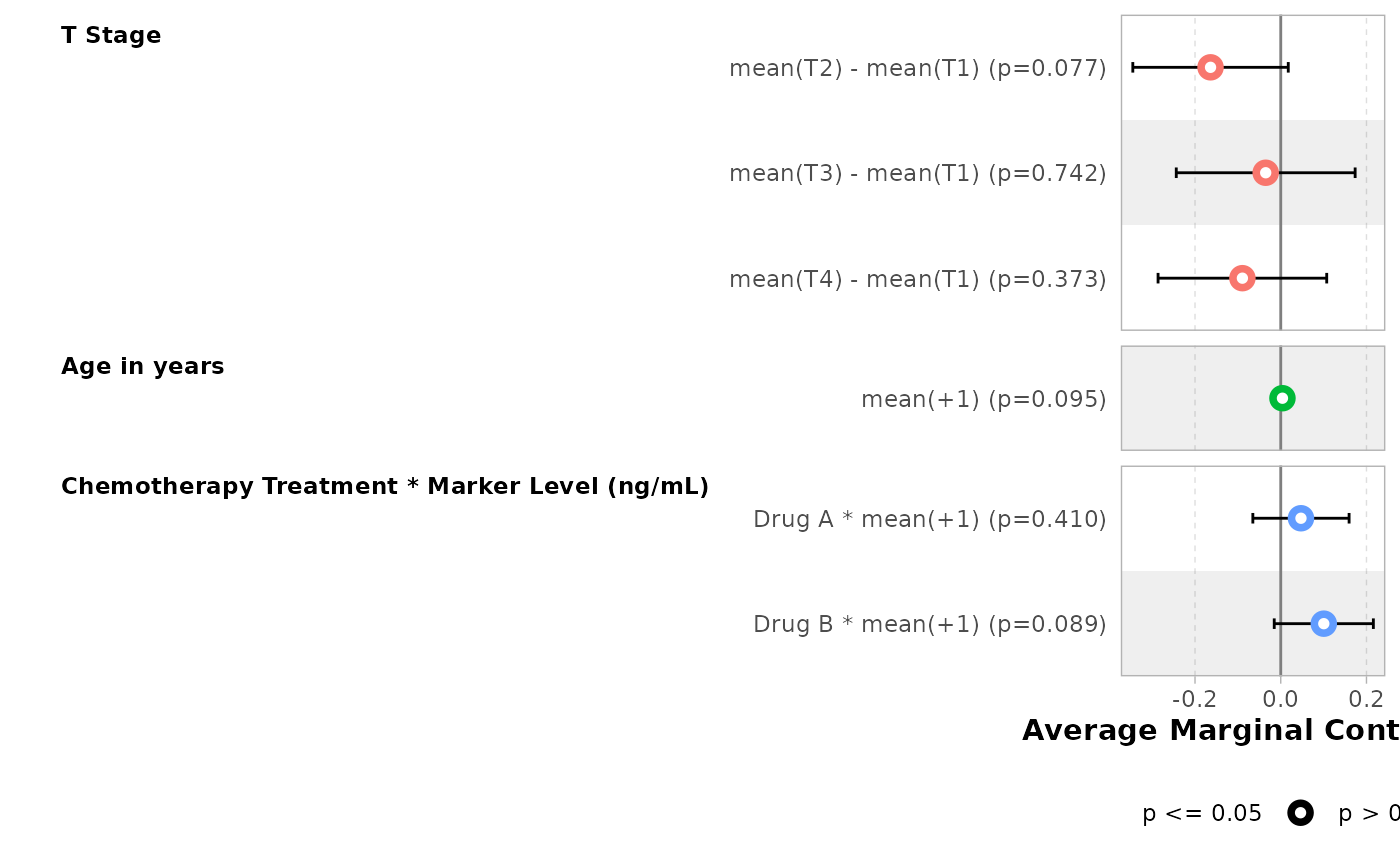
  bold_labels()

Characteristic	Average Marginal Contrasts	95% CI¹	p-value
Age in years
mean(+1)	+0.4%	-0.07%, +0.87%	0.10
Marker Level (ng/mL)
mean(+1)	+7.5%	-0.66%, +15.60%	0.072
T Stage
mean(T2) - mean(T1)	-16.4%	-34.51%, +1.75%	0.077
mean(T3) - mean(T1)	-3.5%	-24.37%, +17.36%	0.7
mean(T4) - mean(T1)	-8.9%	-28.62%, +10.73%	0.4
Chemotherapy Treatment
mean(Drug B) - mean(Drug A)	+6.0%	-7.50%, +19.52%	0.4
¹ CI = Confidence Interval

Similarly, a forest plot could be produced with ggstats::ggcoef_model().

ggstats::ggcoef_model(
  mod,
  tidy_fun = tidy_avg_comparisons,
  variable_labels = c(age = "Age in years")
) +
  ggplot2::scale_x_continuous(
    labels = scales::label_percent(style_positive = "plus")
  )

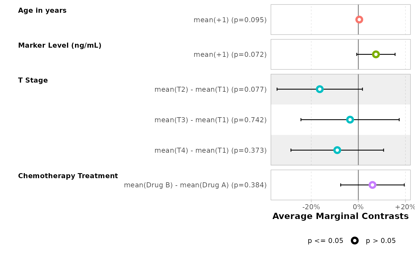
Marginal Contrasts at the Mean

Instead of computing contrasts for each observed values before averaging, another approach consist of considering an hypothetical individual whose characteristics correspond to the “average” before predicting results and computing contrasts.

It could be achieved with marginaleffects by using newdata = "mean". In that case, it will consider an individual where continuous predictors are equal to the mean of observed values and where categorical predictors will be set to the mode (i.e. most frequent value) of the observed values.

pred <- predictions(mod, variables = "trt", newdata = "mean")
pred
#> 
#>  marker stage  age    trt Estimate Pr(>|z|)    S  2.5 % 97.5 %
#>   0.919    T2 46.9 Drug A    0.194  < 0.001 10.8 0.0969  0.351
#>   0.919    T2 46.9 Drug B    0.242  0.00282  8.5 0.1308  0.403
#> 
#> Columns: rowid, rowidcf, estimate, p.value, s.value, conf.low, conf.high, response, marker, stage, age, trt 
#> Type:  invlink(link)
pred$estimate[2] - pred$estimate[1]
#> [1] 0.04738154
comparisons(mod, variables = "trt", newdata = "mean")
#> 
#>  Term        Contrast Estimate Std. Error     z Pr(>|z|)   S  2.5 % 97.5 %
#>   trt Drug B - Drug A   0.0474     0.0579 0.819    0.413 1.3 -0.066  0.161
#>     trt marker stage  age
#>  Drug B  0.919    T2 46.9
#> 
#> Columns: rowid, term, contrast, estimate, std.error, statistic, p.value, s.value, conf.low, conf.high, predicted_lo, predicted_hi, predicted, trt, marker, stage, age, response 
#> Type:  response

The newdata argument can be passed to tidy_avg_comparisons(), tidy_plus_plus or gtsummary::tbl_regression().

mod |>
  tbl_regression(
    tidy_fun = tidy_avg_comparisons,
    newdata = "mean",
    estimate_fun = scales::label_percent(style_positive = "plus"),
    label = list(age = "Age in years")
  ) |>
  bold_labels()

Characteristic	Marginal Contrasts at the Mean	95% CI¹	p-value
Age in years
mean(+1)	+0.4%	-0.1%, +0.8%	0.11
Marker Level (ng/mL)
mean(+1)	+9.2%	-2.6%, +21.0%	0.13
T Stage
mean(T2) - mean(T1)	-17.7%	-37.8%, +2.3%	0.083
mean(T3) - mean(T1)	-3.8%	-26.2%, +18.7%	0.7
mean(T4) - mean(T1)	-9.6%	-30.9%, +11.6%	0.4
Chemotherapy Treatment
mean(Drug B) - mean(Drug A)	+4.7%	-6.6%, +16.1%	0.4
¹ CI = Confidence Interval

For ggstats::ggcoef_model(), use tidy_args to pass newdata = "mean".

mod |>
  ggstats::ggcoef_model(
    tidy_fun = tidy_avg_comparisons,
    tidy_args = list(newdata = "mean"),
    variable_labels = c(age = "Age in years")
  ) +
  ggplot2::scale_x_continuous(
    labels = scales::label_percent(style_positive = "plus")
  )

Alternative approaches

Other assumptions, such as "marginalmeans" or "median", could be defined using newdata. See the documentation of marginaleffects::comparisons().

mod |>
  tbl_regression(
    tidy_fun = tidy_avg_comparisons,
    newdata = "marginalmeans",
    estimate_fun = scales::label_percent(style_positive = "plus"),
    label = list(age = "Age in years")
  ) |>
  bold_labels()

Characteristic	Marginal Contrasts at Marginal Means	95% CI¹	p-value
Age in years
mean(+1)	+0.4%	-0.08%, +0.9%	0.10
Marker Level (ng/mL)
mean(+1)	+7.7%	-0.97%, +16.3%	0.082
T Stage
mean(T2) - mean(T1)	-16.8%	-35.69%, +2.1%	0.082
mean(T3) - mean(T1)	-3.6%	-25.25%, +18.0%	0.7
mean(T4) - mean(T1)	-9.2%	-29.52%, +11.1%	0.4
Chemotherapy Treatment
mean(Drug B) - mean(Drug A)	+5.9%	-8.11%, +19.8%	0.4
¹ CI = Confidence Interval

mod |>
  ggstats::ggcoef_model(
    tidy_fun = tidy_avg_comparisons,
    tidy_args = list(newdata = "marginalmeans"),
    variable_labels = c(age = "Age in years")
  ) +
  ggplot2::scale_x_continuous(
    labels = scales::label_percent(style_positive = "plus")
  )

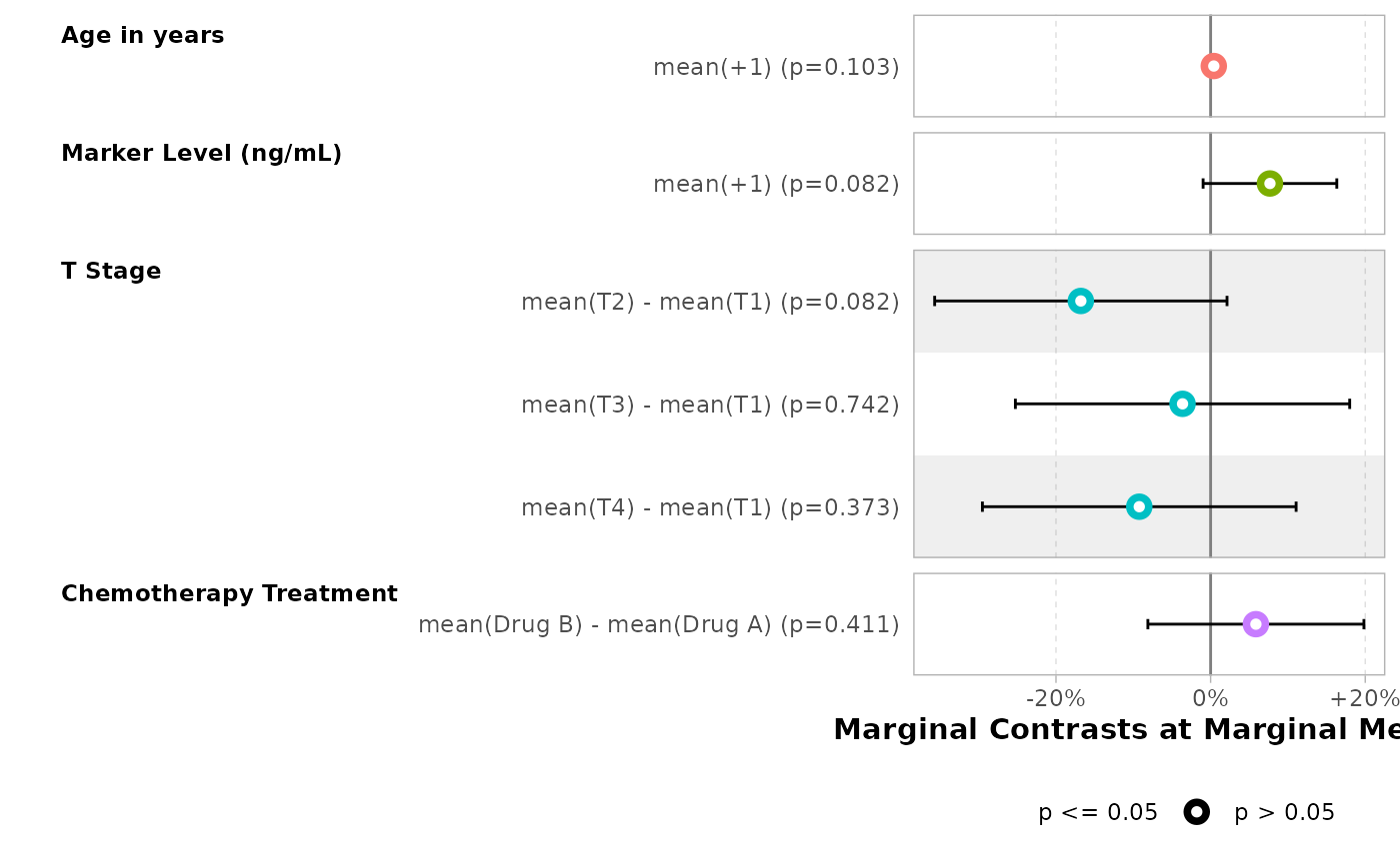
Dealing with interactions

In our model, we defined an interaction between trt and marker. Therefore, we could be interested to compute the contrast of marker for each value of trt.

avg_comparisons(
  mod,
  variables = list(marker = 1),
  newdata = datagrid(
    trt = unique,
    grid_type = "counterfactual"
  ),
  by = "trt"
)
#> 
#>    Term Contrast    trt Estimate Std. Error     z Pr(>|z|)   S   2.5 % 97.5 %
#>  marker mean(+1) Drug A   0.0472     0.0573 0.824   0.4101 1.3 -0.0651  0.159
#>  marker mean(+1) Drug B   0.1004     0.0590 1.703   0.0887 3.5 -0.0152  0.216
#> 
#> Columns: term, contrast, trt, estimate, std.error, statistic, p.value, s.value, conf.low, conf.high, predicted_lo, predicted_hi, predicted 
#> Type:  response

Alternatively, it is possible to compute “cross-contrasts” showing what is happening when both marker and trt are changing.

avg_comparisons(
  mod,
  variables = list(marker = 1, trt = "reference"),
  cross = TRUE
)
#> 
#>  Estimate Std. Error    z Pr(>|z|)   S   2.5 % 97.5 % C: marker
#>     0.161     0.0959 1.67   0.0941 3.4 -0.0274  0.348  mean(+1)
#>                       C: trt
#>  mean(Drug B) - mean(Drug A)
#> 
#> Columns: term, contrast_marker, contrast_trt, estimate, std.error, statistic, p.value, s.value, conf.low, conf.high, predicted_lo, predicted_hi, predicted 
#> Type:  response

The tidier tidy_marginal_contrasts() allows to compute directly several combinations of variables and to stack all the results in a unique tibble.

mod |>
  tbl_regression(
    tidy_fun = tidy_marginal_contrasts,
    estimate_fun = scales::label_percent(style_positive = "plus"),
    label = list(age = "Age in years")
  ) |>
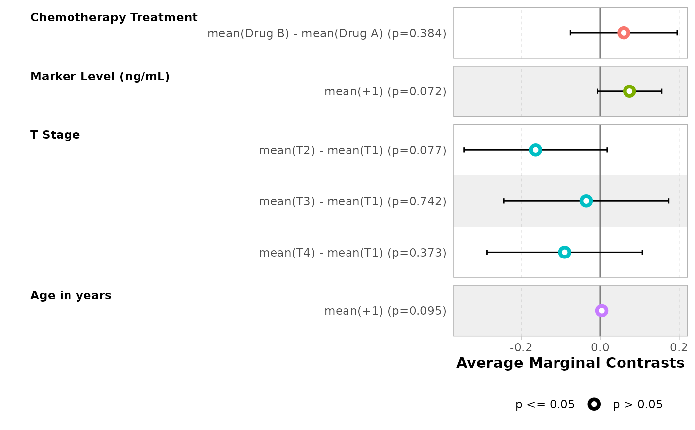
  bold_labels()

Characteristic	Average Marginal Contrasts	95% CI¹	p-value
T Stage
mean(T2) - mean(T1)	-16.4%	-34.5%, +1.75%	0.077
mean(T3) - mean(T1)	-3.5%	-24.4%, +17.36%	0.7
mean(T4) - mean(T1)	-8.9%	-28.6%, +10.73%	0.4
Age in years
mean(+1)	+0.4%	-0.1%, +0.87%	0.10
Chemotherapy Treatment * Marker Level (ng/mL)
Drug A * mean(+1)	+4.7%	-6.5%, +15.95%	0.4
Drug B * mean(+1)	+10.0%	-1.5%, +21.61%	0.089
¹ CI = Confidence Interval

ggstats::ggcoef_model(
  mod,
  tidy_fun = tidy_marginal_contrasts,
  variable_labels = c(age = "Age in years")
)

By default, when there is an interaction, contrasts are computed for the last variable of the interaction according to the different values of the first variables (if one of this variable is continuous, using Tukey’s five numbers).

The option variables_list = "cross" could be used to get “cross-contrasts” for interactions.

mod |>
  tbl_regression(
    tidy_fun = tidy_marginal_contrasts,
    variables_list = "cross",
    estimate_fun = scales::label_percent(style_positive = "plus"),
    label = list(age = "Age in years")
  ) |>
  bold_labels()

Characteristic	Average Marginal Contrasts	95% CI¹	p-value
T Stage
mean(T2) - mean(T1)	-16.4%	-34.5%, +1.75%	0.077
mean(T3) - mean(T1)	-3.5%	-24.4%, +17.36%	0.7
mean(T4) - mean(T1)	-8.9%	-28.6%, +10.73%	0.4
Age in years
mean(+1)	+0.4%	-0.1%, +0.87%	0.10
Chemotherapy Treatment * Marker Level (ng/mL)
mean(+1) * mean(Drug B) - mean(Drug A)	+16.1%	-2.7%, +34.84%	0.094
¹ CI = Confidence Interval

The option variables_list = "no_interaction" could be used to get the average marginal contrasts for each variable without considering interactions.

mod |>
  tbl_regression(
    tidy_fun = tidy_marginal_contrasts,
    variables_list = "no_interaction",
    estimate_fun = scales::label_percent(style_positive = "plus"),
    label = list(age = "Age in years")
  ) |>
  bold_labels()

Characteristic	Average Marginal Contrasts	95% CI¹	p-value
Chemotherapy Treatment
mean(Drug B) - mean(Drug A)	+6.0%	-7.50%, +19.52%	0.4
Marker Level (ng/mL)
mean(+1)	+7.5%	-0.66%, +15.60%	0.072
T Stage
mean(T2) - mean(T1)	-16.4%	-34.51%, +1.75%	0.077
mean(T3) - mean(T1)	-3.5%	-24.37%, +17.36%	0.7
mean(T4) - mean(T1)	-8.9%	-28.62%, +10.73%	0.4
Age in years
mean(+1)	+0.4%	-0.07%, +0.87%	0.10
¹ CI = Confidence Interval

ggstats::ggcoef_model(
  mod,
  tidy_fun = tidy_marginal_contrasts,
  tidy_args = list(variables_list = "no_interaction"),
  variable_labels = c(age = "Age in years")
)

As before, to display marginal contrasts at the mean, indicate newdata = "mean". For more information on the way to customize the combination of variables, see the documentation and examples of tidy_marginal_contrasts().

Marginal Effects / Marginal Slopes

Marginal effects are similar to marginal contrasts with a subtle difference. For a continuous regressor, a marginal contrast could be seen as a difference while a marginal effect is a partial derivative. Put differently, the marginal effect of a continuous regressor $x$ is the slope of the prediction function $y$ , measured at a specific value of $x$ , i.e. ${\partial y}/{\partial x}$ .

Marginal effects are expressed according to the scale of the model and represent the expected change on the outcome for an increase of one unit of the regressor.

By definition, marginal effects are not defined for categorical variables, marginal contrasts being reported instead.

Like marginal contrasts, several approaches exist to compute marginal effects. For more details, see the dedicated vignette of the marginaleffects package.

Average Marginal Effects (AME)

A marginal effect will be computed for each observed values before being averaged with marginaleffects::avg_slopes().

avg_slopes(mod)
#> 
#>    Term                    Contrast Estimate Std. Error      z Pr(>|z|)   S
#>  age    mean(dY/dX)                  0.00397    0.00237  1.679   0.0932 3.4
#>  marker mean(dY/dX)                  0.07104    0.03818  1.861   0.0628 4.0
#>  stage  mean(T2) - mean(T1)         -0.16378    0.09252 -1.770   0.0767 3.7
#>  stage  mean(T3) - mean(T1)         -0.03509    0.10646 -0.330   0.7417 0.4
#>  stage  mean(T4) - mean(T1)         -0.08947    0.10037 -0.891   0.3727 1.4
#>  trt    mean(Drug B) - mean(Drug A)  0.06006    0.06893  0.871   0.3836 1.4
#>      2.5 %  97.5 %
#>  -0.000666 0.00861
#>  -0.003781 0.14587
#>  -0.345109 0.01755
#>  -0.243740 0.17356
#>  -0.286204 0.10726
#>  -0.075043 0.19517
#> 
#> Columns: term, contrast, estimate, std.error, statistic, p.value, s.value, conf.low, conf.high, predicted_lo, predicted_hi, predicted 
#> Type:  response

Column names are not consistent with other tidiers used by broom.helpers. Use tidy_avg_slopes() instead.

mod |>
  tbl_regression(
    tidy_fun = tidy_avg_slopes,
    estimate_fun = scales::label_percent(style_positive = "plus"),
    label = list(age = "Age in years")
  ) |>
  bold_labels()

Characteristic	Average Marginal Effects	95% CI¹	p-value
Age in years
mean(dY/dX)	+0.4%	-0.07%, +0.86%	0.093
Marker Level (ng/mL)
mean(dY/dX)	+7.1%	-0.38%, +14.59%	0.063
T Stage
mean(T2) - mean(T1)	-16.4%	-34.51%, +1.75%	0.077
mean(T3) - mean(T1)	-3.5%	-24.37%, +17.36%	0.7
mean(T4) - mean(T1)	-8.9%	-28.62%, +10.73%	0.4
Chemotherapy Treatment
mean(Drug B) - mean(Drug A)	+6.0%	-7.50%, +19.52%	0.4
¹ CI = Confidence Interval

mod |>
  ggstats::ggcoef_model(
    tidy_fun = tidy_avg_slopes,
    variable_labels = c(age = "Age in years")
  ) +
  ggplot2::scale_x_continuous(
    labels = scales::label_percent(style_positive = "plus")
  )

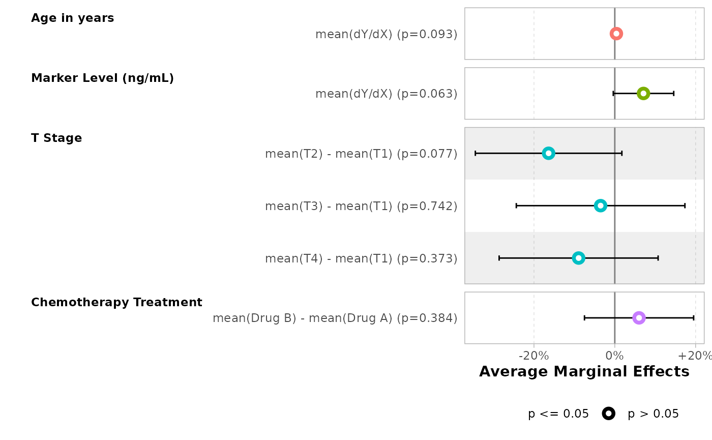
Please note that for categorical variables, marginal contrasts are returned.

Same results could be obtained with margins::margins() function inspired by Stata’s margins command. As margins::margins() is not compatible with stats::poly(), we will rewrite our model, replacing poly(age, 2) by age + age^2.

mod_alt <- glm(
  response ~ trt * marker + stage + age + age^2,
  data = d,
  family = binomial
)
margins::margins(mod_alt) |> tidy()
#> Warning: tidying a `margins` object was deprecated in broom 1.0.6.
#> ℹ margins was removed from CRAN in April 2024 and its tidiers are thus
#>   untested.
#> ! Please interpret output with caution.
#> This warning is displayed once every 8 hours.
#> Call `lifecycle::last_lifecycle_warnings()` to see where this warning was
#> generated.
#> # A tibble: 6 × 5
#>   term      estimate std.error statistic p.value
#>   <chr>        <dbl>     <dbl>     <dbl>   <dbl>
#> 1 age        0.00397   0.00236     1.68   0.0927
#> 2 marker     0.0710    0.0380      1.87   0.0617
#> 3 stageT2   -0.164     0.0922     -1.78   0.0754
#> 4 stageT3   -0.0351    0.106      -0.330  0.742 
#> 5 stageT4   -0.0895    0.100      -0.891  0.373 
#> 6 trtDrug B  0.0600    0.0689      0.871  0.384

For broom.helpers, gtsummary or ggstats, use tidy_margins().

mod_alt |>
  tbl_regression(
    tidy_fun = tidy_margins,
    estimate_fun = scales::label_percent(style_positive = "plus")
  ) |>
  bold_labels()

Characteristic	Average Marginal Effects	95% CI¹	p-value
Age	+0.4%	-0.07%, +0.86%	0.093
Marker Level (ng/mL)	+7.1%	-0.35%, +14.55%	0.062
T Stage
T1	—	—
T2	-16.4%	-34.46%, +1.68%	0.075
T3	-3.5%	-24.37%, +17.35%	0.7
T4	-8.9%	-28.62%, +10.73%	0.4
Chemotherapy Treatment
Drug A	—	—
Drug B	+6.0%	-7.50%, +19.51%	0.4
¹ CI = Confidence Interval

Marginal Effects at the Mean (MEM)

For marginal effects at the mean², simple use newdata = "mean".

mod |>
  tbl_regression(
    tidy_fun = tidy_avg_slopes,
    newdata = "mean",
    estimate_fun = scales::label_percent(style_positive = "plus"),
    label = list(age = "Age in years")
  ) |>
  bold_labels()

Characteristic	Marginal Effects at the Mean	95% CI¹	p-value
Age in years
mean(dY/dX)	+0.4%	-0.1%, +0.80%	0.11
Marker Level (ng/mL)
mean(dY/dX)	+8.3%	-1.6%, +18.17%	0.10
T Stage
mean(T2) - mean(T1)	-17.7%	-37.8%, +2.34%	0.083
mean(T3) - mean(T1)	-3.8%	-26.2%, +18.67%	0.7
mean(T4) - mean(T1)	-9.6%	-30.9%, +11.60%	0.4
Chemotherapy Treatment
mean(Drug B) - mean(Drug A)	+4.7%	-6.6%, +16.08%	0.4
¹ CI = Confidence Interval

mod |>
  ggstats::ggcoef_model(
    tidy_fun = tidy_avg_slopes,
    tidy_args = list(newdata = "mean"),
    variable_labels = c(age = "Age in years")
  ) +
  ggplot2::scale_x_continuous(
    labels = scales::label_percent(style_positive = "plus")
  )

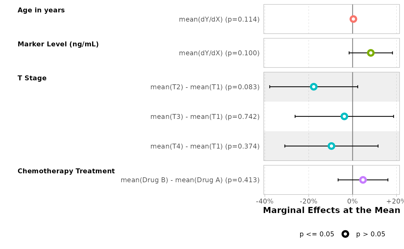
Marginal Effects at Marginal Means

Simply use newdata = "marginalmeans".

mod |>
  tbl_regression(
    tidy_fun = tidy_avg_slopes,
    newdata = "marginalmeans",
    estimate_fun = scales::label_percent(style_positive = "plus"),
    label = list(age = "Age in years")
  ) |>
  bold_labels()

Characteristic	Marginal Effects at Marginal Means	95% CI¹	p-value
Age in years
mean(dY/dX)	+0.4%	-0.08%, +0.9%	0.10
Marker Level (ng/mL)
mean(dY/dX)	+7.3%	-0.63%, +15.2%	0.071
T Stage
mean(T2) - mean(T1)	-16.8%	-35.69%, +2.1%	0.082
mean(T3) - mean(T1)	-3.6%	-25.25%, +18.0%	0.7
mean(T4) - mean(T1)	-9.2%	-29.52%, +11.1%	0.4
Chemotherapy Treatment
mean(Drug B) - mean(Drug A)	+5.9%	-8.11%, +19.8%	0.4
¹ CI = Confidence Interval

mod |>
  ggstats::ggcoef_model(
    tidy_fun = tidy_avg_slopes,
    tidy_args = list(newdata = "marginalmeans"),
    variable_labels = c(age = "Age in years")
  ) +
  ggplot2::scale_x_continuous(
    labels = scales::label_percent(style_positive = "plus")
  )

Terminology

Data preparation

Marginal Predictions

Marginal Predictions at the Mean

the {effects}’s approach

the {marginaleffects}’s approach at the Mean

Average Marginal Predictions

Marginal Means and Marginal Predictions at Marginal Means

Alternative approaches

Marginal Predictions at the Median

the ggeffects::ggpredict()’s approach

Marginal Contrasts

Average Marginal Contrasts

Marginal Contrasts at the Mean

Alternative approaches

Dealing with interactions

Marginal Effects / Marginal Slopes

Average Marginal Effects (AME)

Marginal Effects at the Mean (MEM)

Marginal Effects at Marginal Means

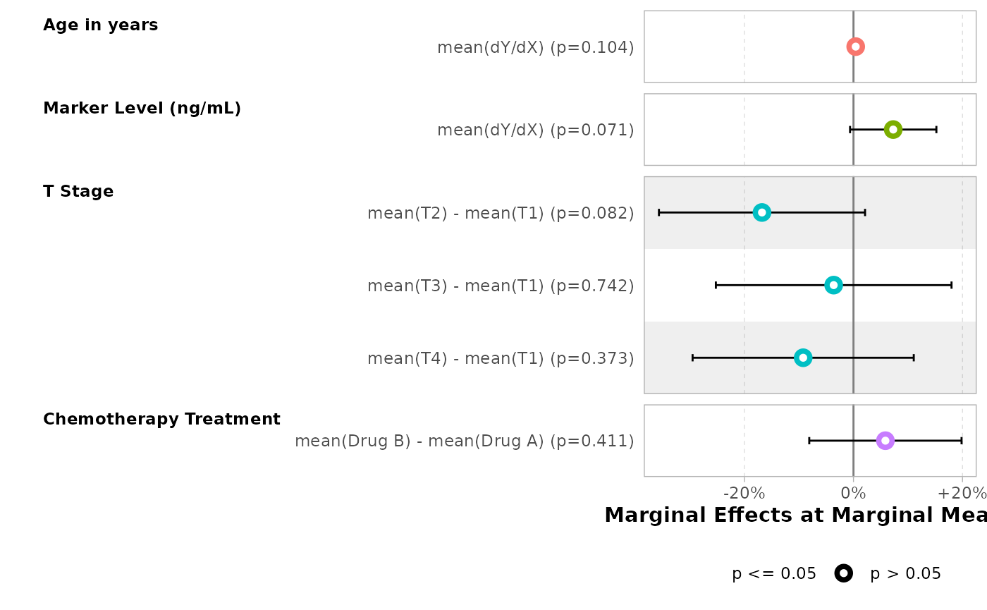
Further readings

the `{effects}`’s approach

the `{marginaleffects}`’s approach at the Mean

the `ggeffects::ggpredict()`’s approach