Compute cross-tabulation statistics with `stat

library(ggstats)
#> Error in get(paste0(generic, ".", class), envir = get_method_env()) : 
#>   object 'type_sum.accel' not found
library(ggplot2)

This statistic is intended to be used with two discrete variables mapped to x and y aesthetics. It will compute several statistics of a cross-tabulated table using broom::tidy.test() and stats::chisq.test(). More precisely, the computed variables are:

observed: number of observations in x,y
prop: proportion of total
row.prop: row proportion
col.prop: column proportion
expected: expected count under the null hypothesis
resid: Pearson’s residual
std.resid: standardized residual
row.observed: total number of observations within row
col.observed: total number of observations within column
total.observed: total number of observations within the table
phi: phi coefficients, see augment_chisq_add_phi()

By default, stat_cross() is using ggplot2::geom_points(). If you want to plot the number of observations, you need to map after_stat(observed) to an aesthetic (here size):

d <- as.data.frame(Titanic)
ggplot(d) +
  aes(x = Class, y = Survived, weight = Freq, size = after_stat(observed)) +
  stat_cross() +
  scale_size_area(max_size = 20)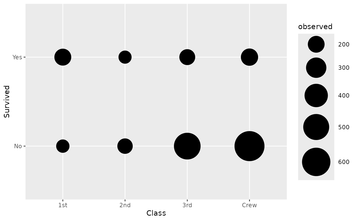

Note that the weight aesthetic is taken into account by stat_cross().

We can go further using a custom shape and filling points with standardized residual to identify visually cells who are over- or underrepresented.

ggplot(d) +
  aes(
    x = Class, y = Survived, weight = Freq,
    size = after_stat(observed), fill = after_stat(std.resid)
  ) +
  stat_cross(shape = 22) +
  scale_fill_steps2(breaks = c(-3, -2, 2, 3), show.limits = TRUE) +
  scale_size_area(max_size = 20)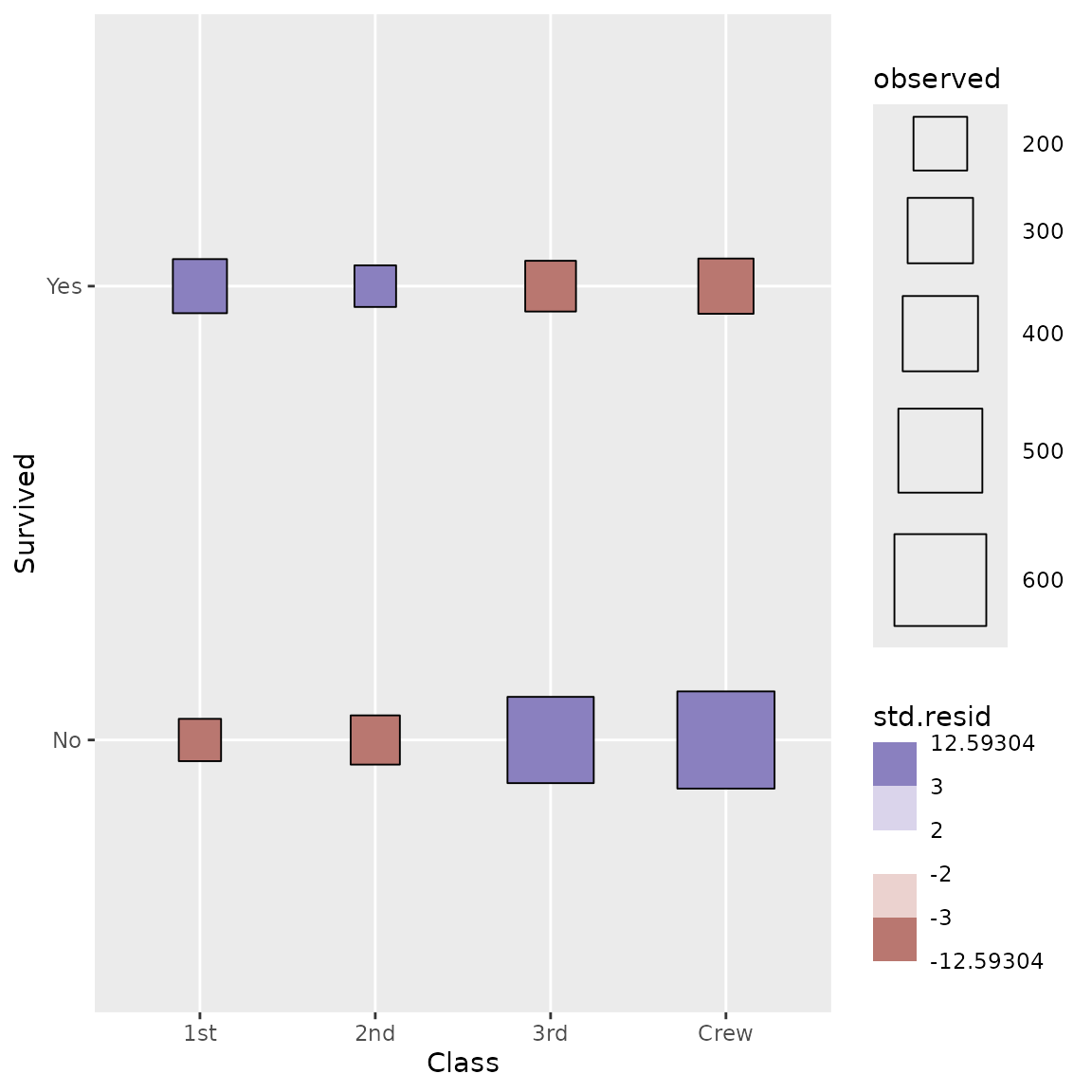

We can easily recreate a cross-tabulated table.

ggplot(d) +
  aes(x = Class, y = Survived, weight = Freq) +
  geom_tile(fill = "white", colour = "black") +
  geom_text(stat = "cross", mapping = aes(label = after_stat(observed))) +
  theme_minimal()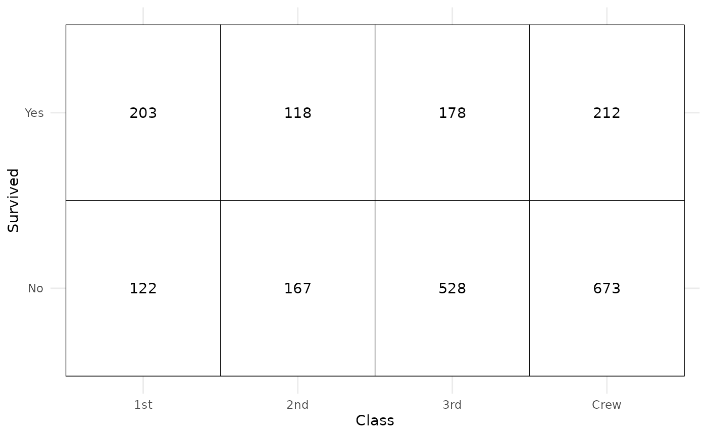

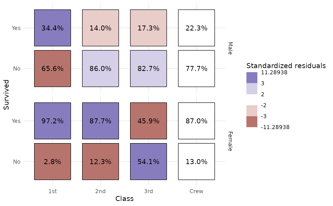
Even more complicated, we want to produce a table showing column proportions and where cells are filled with standardized residuals. Note that stat_cross() could be used with facets. In that case, computation is done separately in each facet.

ggplot(d) +
  aes(
    x = Class, y = Survived, weight = Freq,
    label = scales::percent(after_stat(col.prop), accuracy = .1),
    fill = after_stat(std.resid)
  ) +
  stat_cross(shape = 22, size = 30) +
  geom_text(stat = "cross") +
  scale_fill_steps2(breaks = c(-3, -2, 2, 3), show.limits = TRUE) +
  facet_grid(rows = vars(Sex)) +
  labs(fill = "Standardized residuals") +
  theme_minimal()

Compute cross-tabulation statistics with `stat_cross()`