Plot one or several proportions (defined by logical conditions) by
sub-groups. See proportion() for more details on the way proportions and
confidence intervals are computed. By default, return a bar plot, but other
geometries could be used (see examples). stratified_by() is an helper
function facilitating a stratified analyses (i.e. proportions by groups
stratified according to a third variable, see examples).
dummy_proportions() is an helper to easily convert a categorical variable
into dummy variables and therefore showing the proportion of each level of
the original variable (see examples).
Usage
plot_proportions(
  data,
  condition,
  by = NULL,
  drop_na_by = FALSE,
  convert_continuous = TRUE,
  geom = "bar",
  ...,
  show_overall = TRUE,
  overall_label = "Overall",
  show_ci = TRUE,
  conf_level = 0.95,
  ci_color = "black",
  show_pvalues = TRUE,
  pvalues_test = c("fisher", "chisq"),
  pvalues_labeller = scales::label_pvalue(add_p = TRUE),
  pvalues_size = 3.5,
  show_labels = TRUE,
  label_y = NULL,
  labels_labeller = scales::label_percent(1),
  labels_size = 3.5,
  labels_color = "black",
  show_overall_line = FALSE,
  overall_line_type = "dashed",
  overall_line_color = "black",
  overall_line_width = 0.5,
  facet_labeller = ggplot2::label_wrap_gen(width = 50, multi_line = TRUE),
  flip = FALSE,
  minimal = FALSE,
  free_scale = FALSE,
  return_data = FALSE
)

stratified_by(condition, strata)

dummy_proportions(variable)
Arguments
- data
A data frame, data frame extension (e.g. a tibble), or a survey design object.
- condition
<
data-masking>
A condition defining a proportion, or adplyr::tibble()defining several proportions (see examples).- by
<
tidy-select>
List of variables to group by (comparison is done separately for each variable).- drop_na_by
Remove
NAvalues inbyvariables?- convert_continuous
Should continuous by variables (with 5 unique values or more) be converted to quartiles (using
cut_quartiles())?- geom
Geometry to use for plotting proportions (
"bar"by default).- ...
Additional arguments passed to the geom defined by
geom.- show_overall
Display "Overall" column?
- overall_label
Label for the overall column.
- show_ci
Display confidence intervals?
- conf_level
Confidence level for the confidence intervals.
- ci_color
Color of the error bars representing confidence intervals.
- show_pvalues
Display p-values in the top-left corner?
- pvalues_test
Test to compute p-values for data frames:
"fisher"forstats::fisher.test()(withsimulate.p.value = TRUE) or"chisq"forstats::chisq.test(). Has no effect on survey objects for thosesurvey::svychisq()is used.- pvalues_labeller
Labeller function for p-values.
- pvalues_size
Text size for p-values.
- show_labels
Display proportion labels?
- label_y
Y position of labels. If
NULL, will be auto-determined.- labels_labeller
Labeller function for labels.
- labels_size
Size of labels.
- labels_color
Color of labels.
- show_overall_line
Add an overall line?
- overall_line_type
Line type of the overall line.
- overall_line_color
Color of the overall line.
- overall_line_width
Line width of the overall line.
- facet_labeller
Labeller function for strip labels.
- flip
Flip x and y axis?
- minimal
Should a minimal theme be applied? (no y-axis, no grid)
- free_scale
Allow y axis to vary between conditions?
- return_data
Return computed data instead of the plot?
- strata
Stratification variable
- variable
Variable to be converted into dummy variables.
Examples
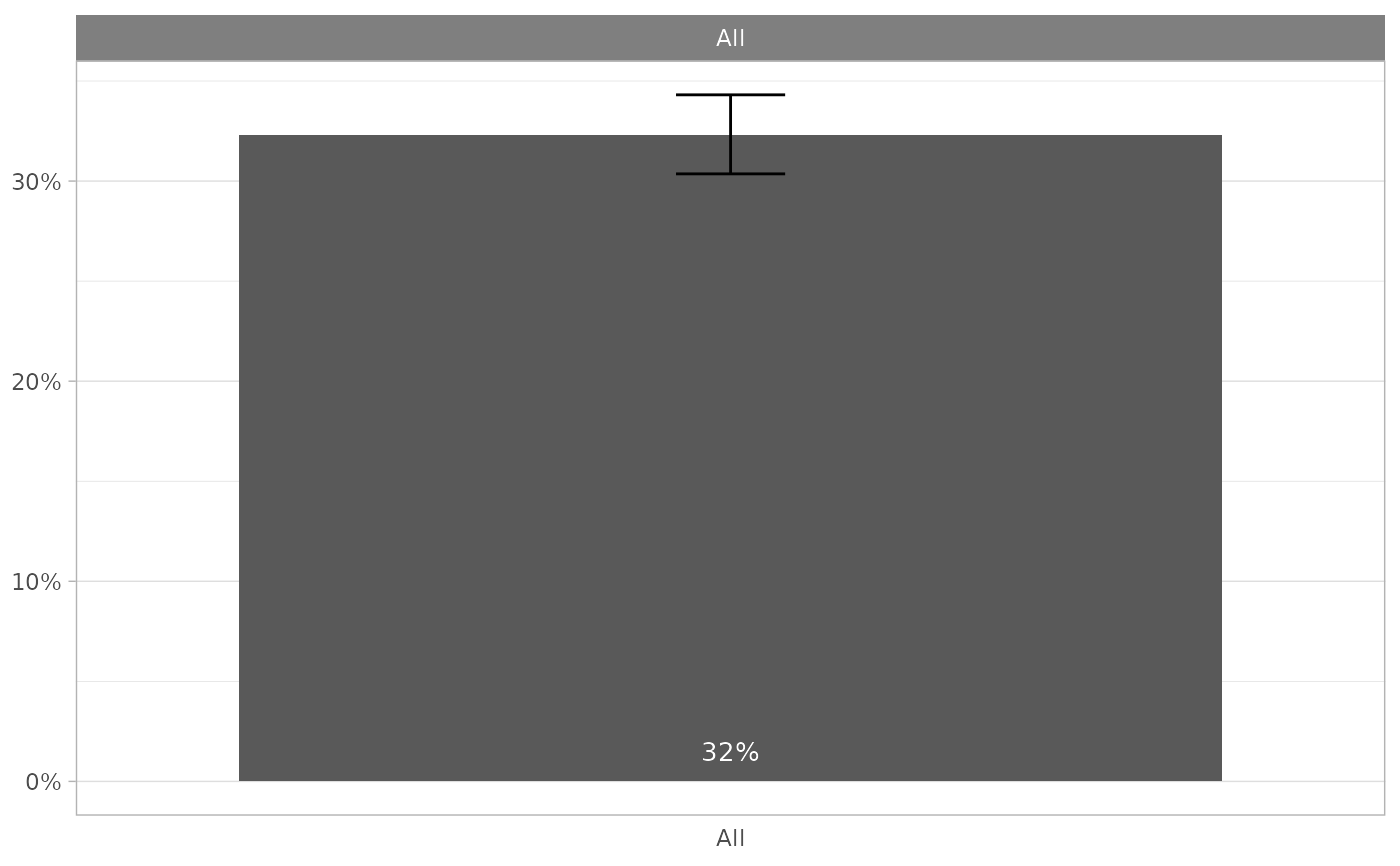
titanic |>
plot_proportions(
Survived == "Yes",
overall_label = "All",
labels_color = "white"
)
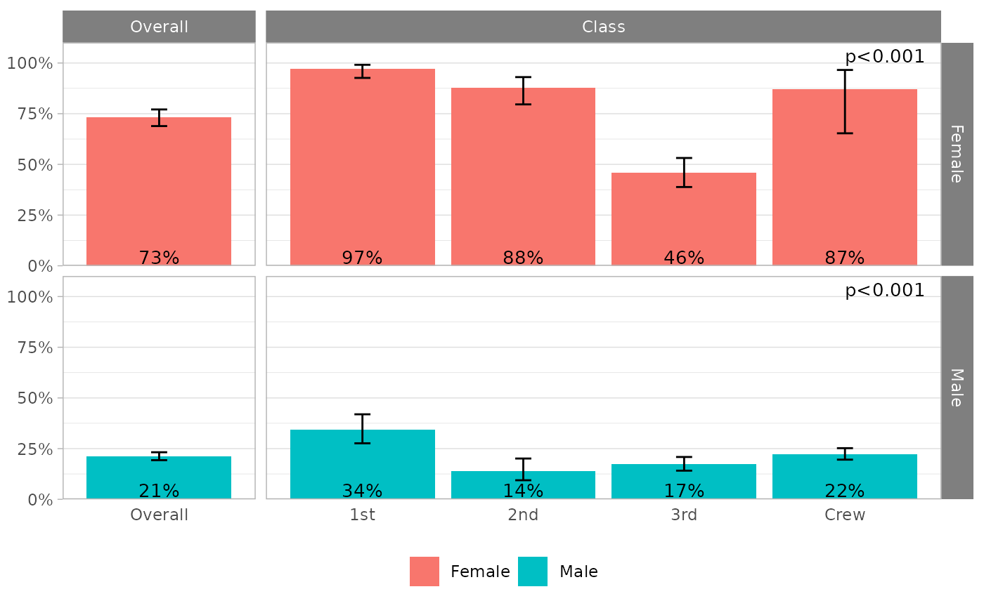
 # \donttest{
titanic |>
plot_proportions(
Survived == "Yes",
by = c(Class, Sex),
fill = "lightblue"
)
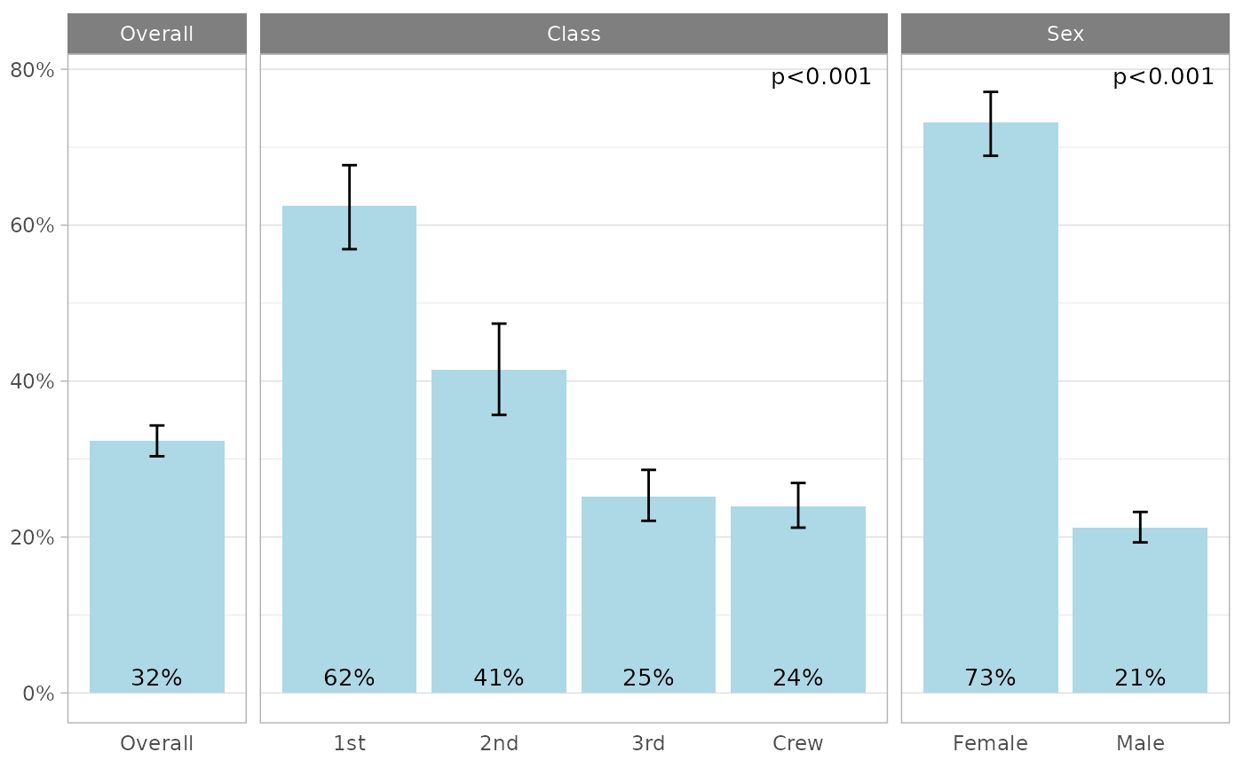
# \donttest{
titanic |>
plot_proportions(
Survived == "Yes",
by = c(Class, Sex),
fill = "lightblue"
)
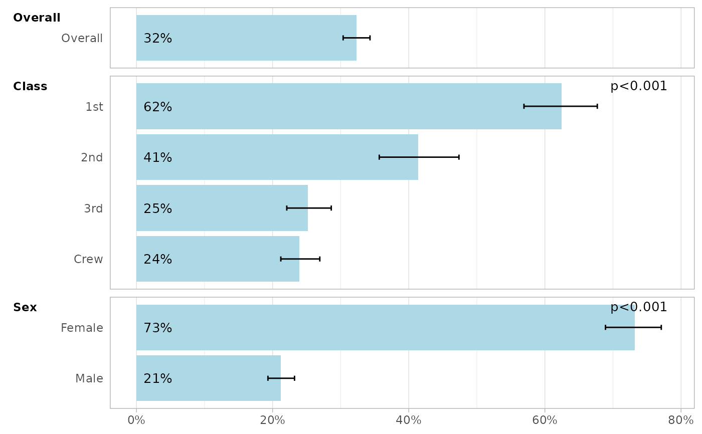
 titanic |>
plot_proportions(
Survived == "Yes",
by = c(Class, Sex),
fill = "lightblue",
flip = TRUE
)
titanic |>
plot_proportions(
Survived == "Yes",
by = c(Class, Sex),
fill = "lightblue",
flip = TRUE
)
 titanic |>
plot_proportions(
Survived == "Yes",
by = c(Class, Sex),
fill = "lightblue",
minimal = TRUE
)
titanic |>
plot_proportions(
Survived == "Yes",
by = c(Class, Sex),
fill = "lightblue",
minimal = TRUE
)
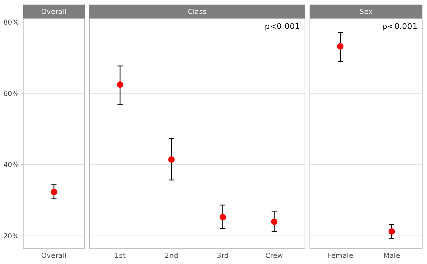 titanic |>
plot_proportions(
Survived == "Yes",
by = c(Class, Sex),
geom = "point",
color = "red",
size = 3,
show_labels = FALSE
)
titanic |>
plot_proportions(
Survived == "Yes",
by = c(Class, Sex),
geom = "point",
color = "red",
size = 3,
show_labels = FALSE
)
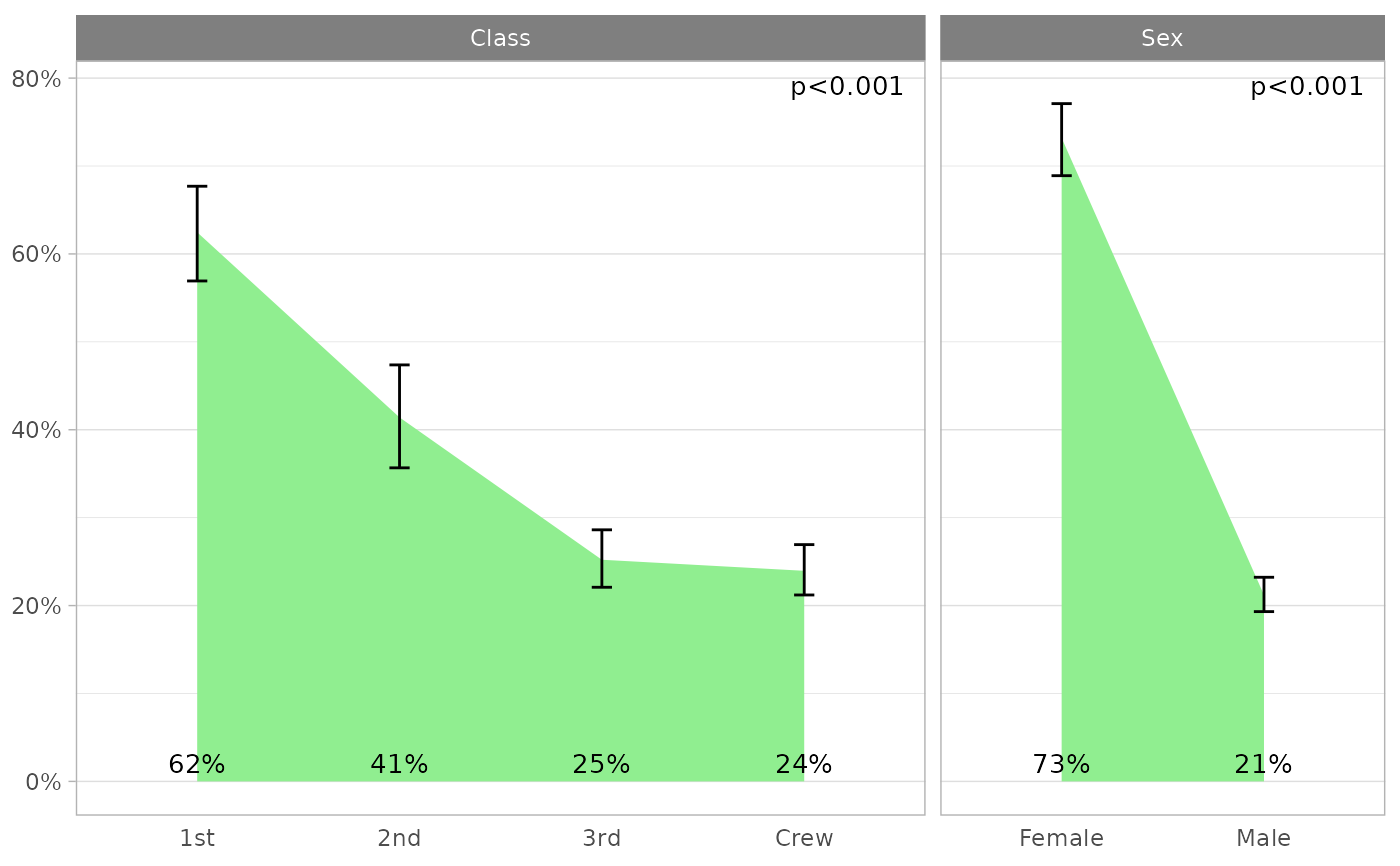 titanic |>
plot_proportions(
Survived == "Yes",
by = c(Class, Sex),
geom = "area",
fill = "lightgreen",
show_overall = FALSE
)
titanic |>
plot_proportions(
Survived == "Yes",
by = c(Class, Sex),
geom = "area",
fill = "lightgreen",
show_overall = FALSE
)
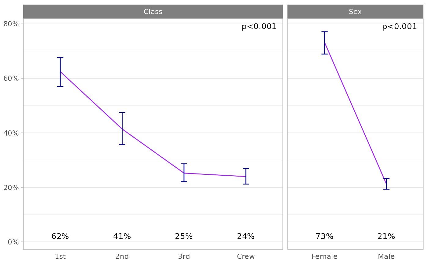 titanic |>
plot_proportions(
Survived == "Yes",
by = c(Class, Sex),
geom = "line",
color = "purple",
ci_color = "darkblue",
show_overall = FALSE
)
titanic |>
plot_proportions(
Survived == "Yes",
by = c(Class, Sex),
geom = "line",
color = "purple",
ci_color = "darkblue",
show_overall = FALSE
)
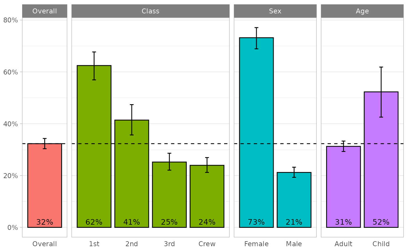 titanic |>
plot_proportions(
Survived == "Yes",
by = -Survived,
mapping = ggplot2::aes(fill = by),
color = "black",
show.legend = FALSE,
show_overall_line = TRUE,
show_pvalues = FALSE
)
titanic |>
plot_proportions(
Survived == "Yes",
by = -Survived,
mapping = ggplot2::aes(fill = by),
color = "black",
show.legend = FALSE,
show_overall_line = TRUE,
show_pvalues = FALSE
)
 # defining several proportions
titanic |>
plot_proportions(
dplyr::tibble(
Survived = Survived == "Yes",
Male = Sex == "Male"
),
by = c(Class),
mapping = ggplot2::aes(fill = condition)
)
# defining several proportions
titanic |>
plot_proportions(
dplyr::tibble(
Survived = Survived == "Yes",
Male = Sex == "Male"
),
by = c(Class),
mapping = ggplot2::aes(fill = condition)
)
 titanic |>
plot_proportions(
dplyr::tibble(
Survived = Survived == "Yes",
Male = Sex == "Male"
),
by = c(Class),
mapping = ggplot2::aes(fill = condition),
free_scale = TRUE
)
titanic |>
plot_proportions(
dplyr::tibble(
Survived = Survived == "Yes",
Male = Sex == "Male"
),
by = c(Class),
mapping = ggplot2::aes(fill = condition),
free_scale = TRUE
)
 iris |>
plot_proportions(
dplyr::tibble(
"Long sepal" = Sepal.Length > 6,
"Short petal" = Petal.Width < 1
),
by = Species,
fill = "palegreen"
)
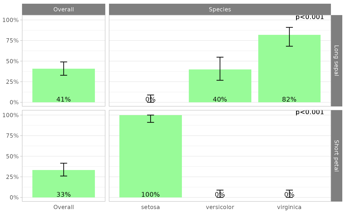
iris |>
plot_proportions(
dplyr::tibble(
"Long sepal" = Sepal.Length > 6,
"Short petal" = Petal.Width < 1
),
by = Species,
fill = "palegreen"
)
 iris |>
plot_proportions(
dplyr::tibble(
"Long sepal" = Sepal.Length > 6,
"Short petal" = Petal.Width < 1
),
by = Species,
fill = "palegreen",
flip = TRUE
)
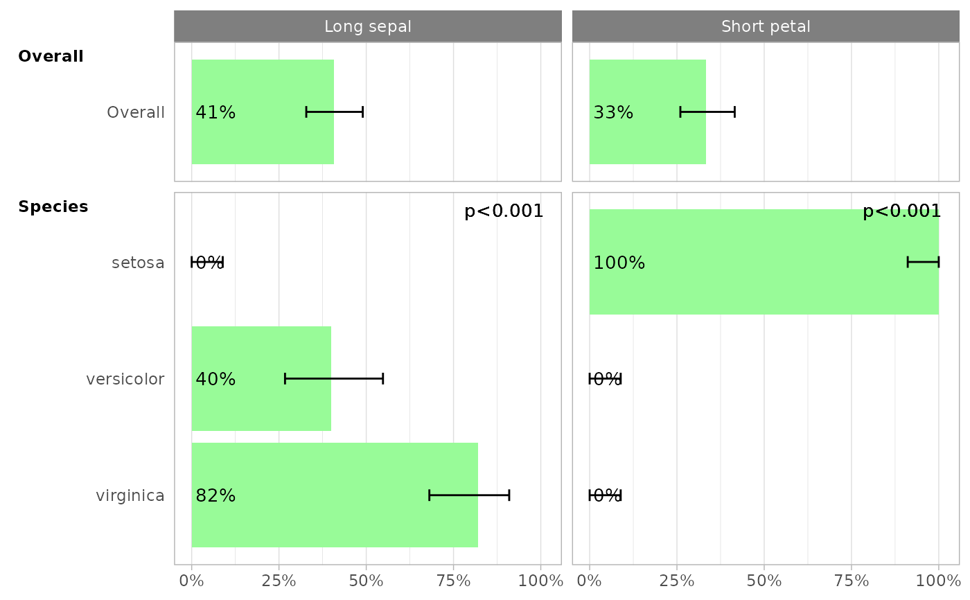
iris |>
plot_proportions(
dplyr::tibble(
"Long sepal" = Sepal.Length > 6,
"Short petal" = Petal.Width < 1
),
by = Species,
fill = "palegreen",
flip = TRUE
)
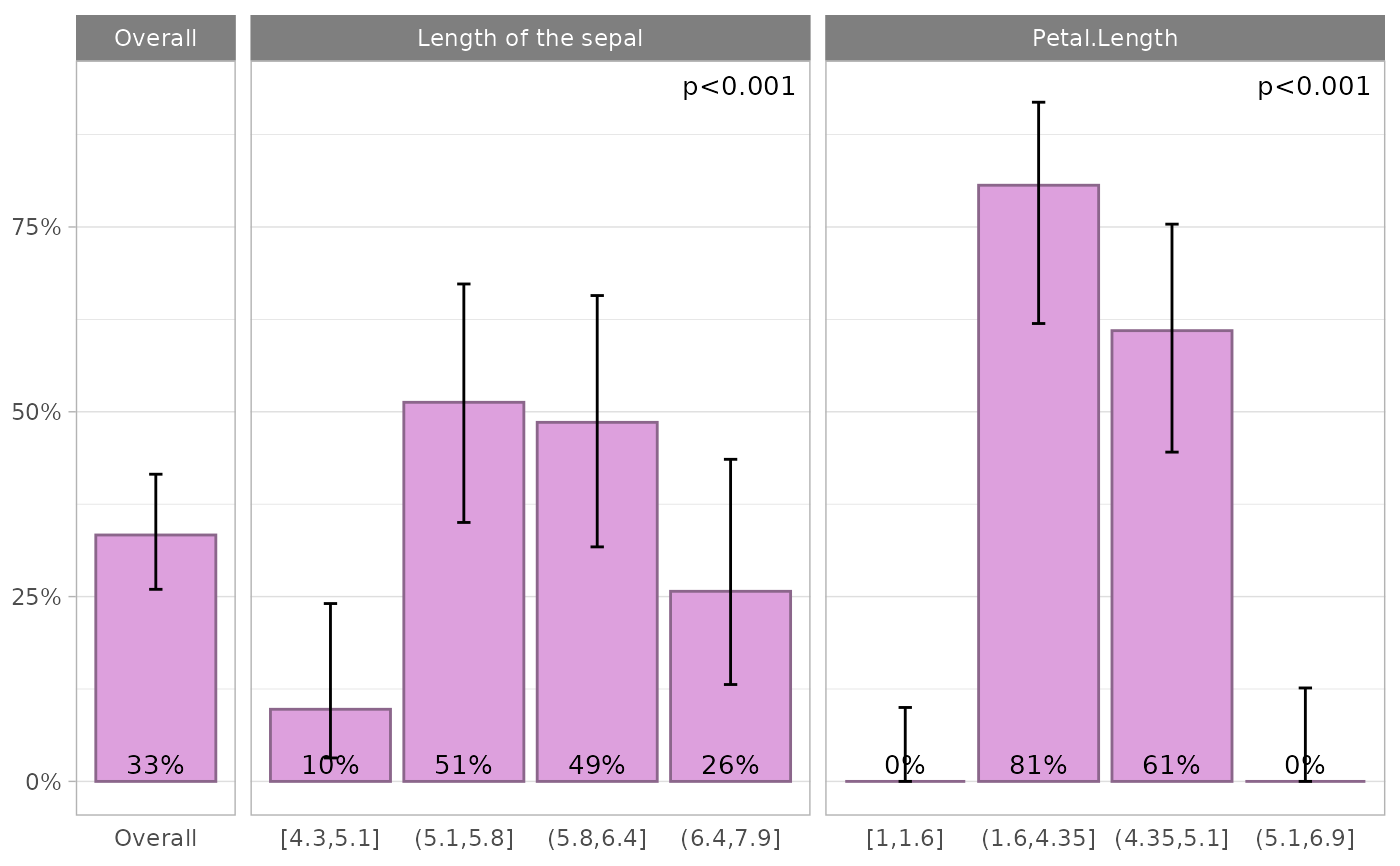
 # works with continuous by variables
iris |>
labelled::set_variable_labels(
Sepal.Length = "Length of the sepal"
) |>
plot_proportions(
Species == "versicolor",
by = dplyr::contains("leng"),
fill = "plum",
colour = "plum4"
)
# works with continuous by variables
iris |>
labelled::set_variable_labels(
Sepal.Length = "Length of the sepal"
) |>
plot_proportions(
Species == "versicolor",
by = dplyr::contains("leng"),
fill = "plum",
colour = "plum4"
)
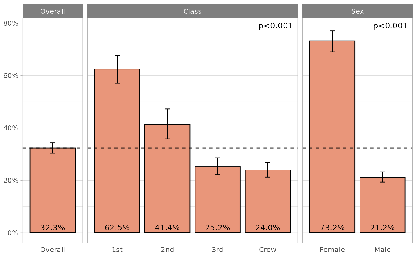
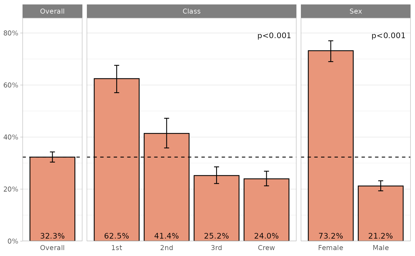 # works with survey object
titanic |>
srvyr::as_survey() |>
plot_proportions(
Survived == "Yes",
by = c(Class, Sex),
fill = "darksalmon",
color = "black",
show_overall_line = TRUE,
labels_labeller = scales::label_percent(.1)
)
# works with survey object
titanic |>
srvyr::as_survey() |>
plot_proportions(
Survived == "Yes",
by = c(Class, Sex),
fill = "darksalmon",
color = "black",
show_overall_line = TRUE,
labels_labeller = scales::label_percent(.1)
)
 # }
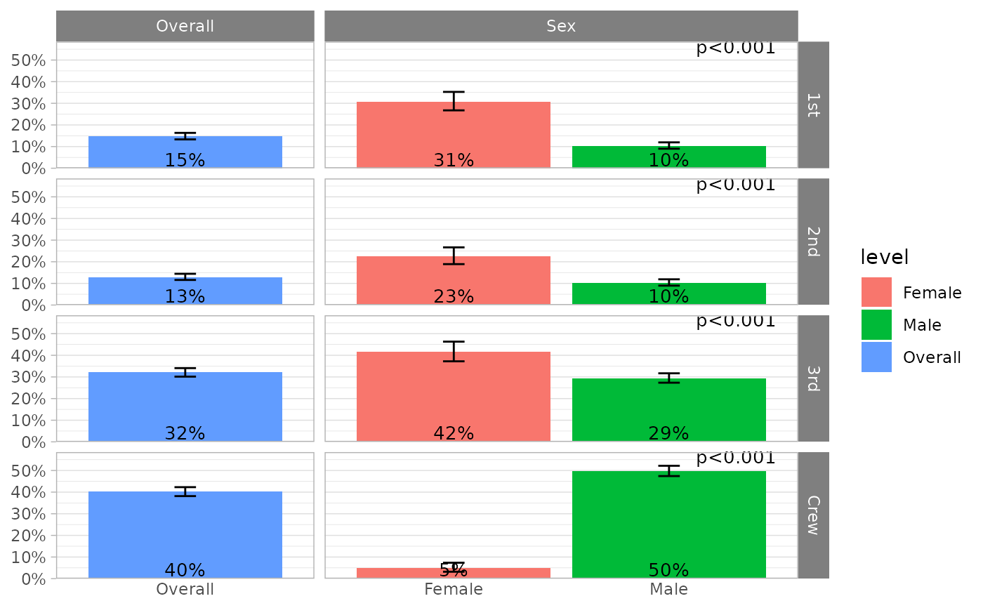
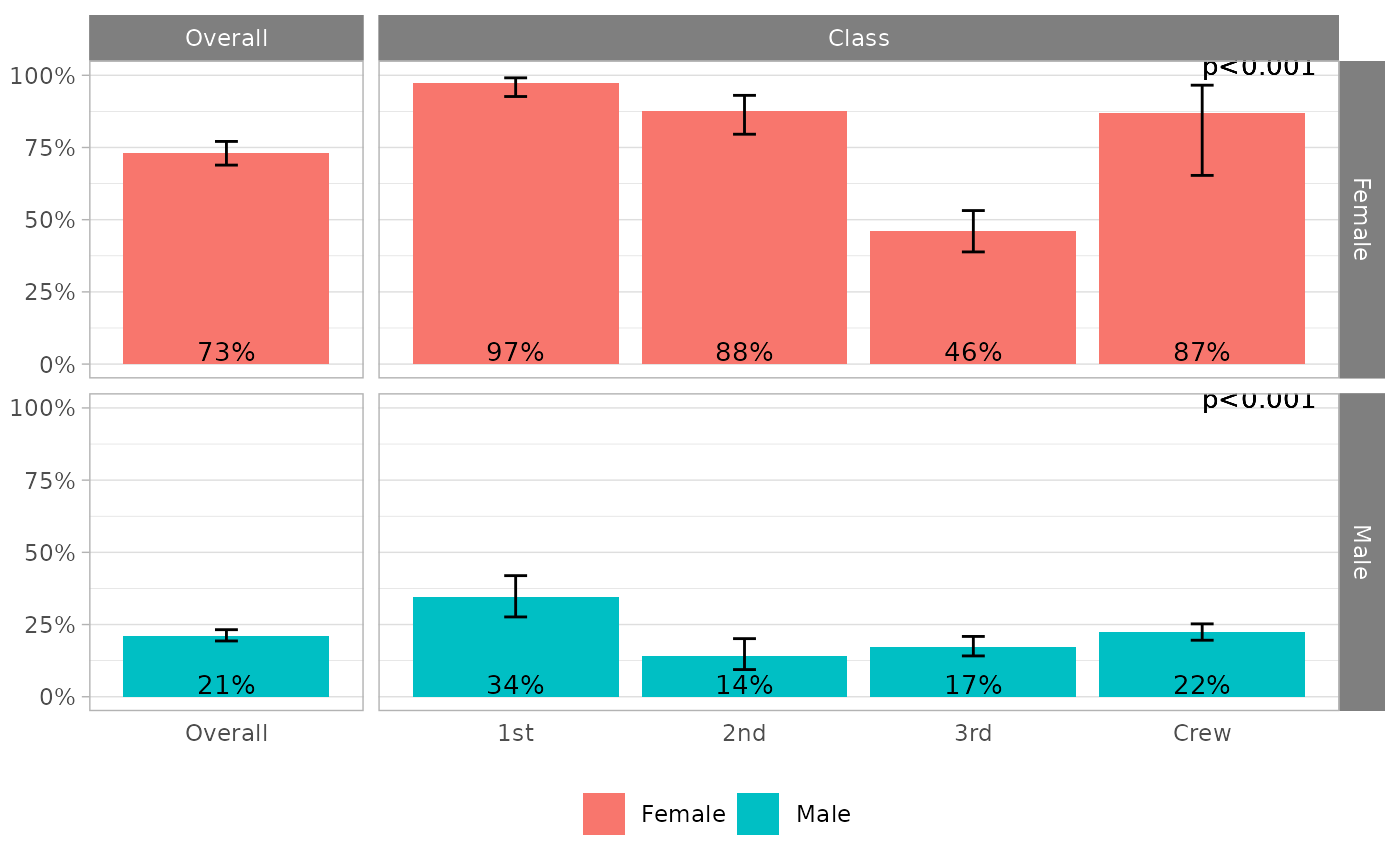
# stratified analysis
titanic |>
plot_proportions(
(Survived == "Yes") |> stratified_by(Sex),
by = Class,
mapping = ggplot2::aes(fill = condition)
) +
ggplot2::theme(legend.position = "bottom") +
ggplot2::labs(fill = NULL)
# }
# stratified analysis
titanic |>
plot_proportions(
(Survived == "Yes") |> stratified_by(Sex),
by = Class,
mapping = ggplot2::aes(fill = condition)
) +
ggplot2::theme(legend.position = "bottom") +
ggplot2::labs(fill = NULL)
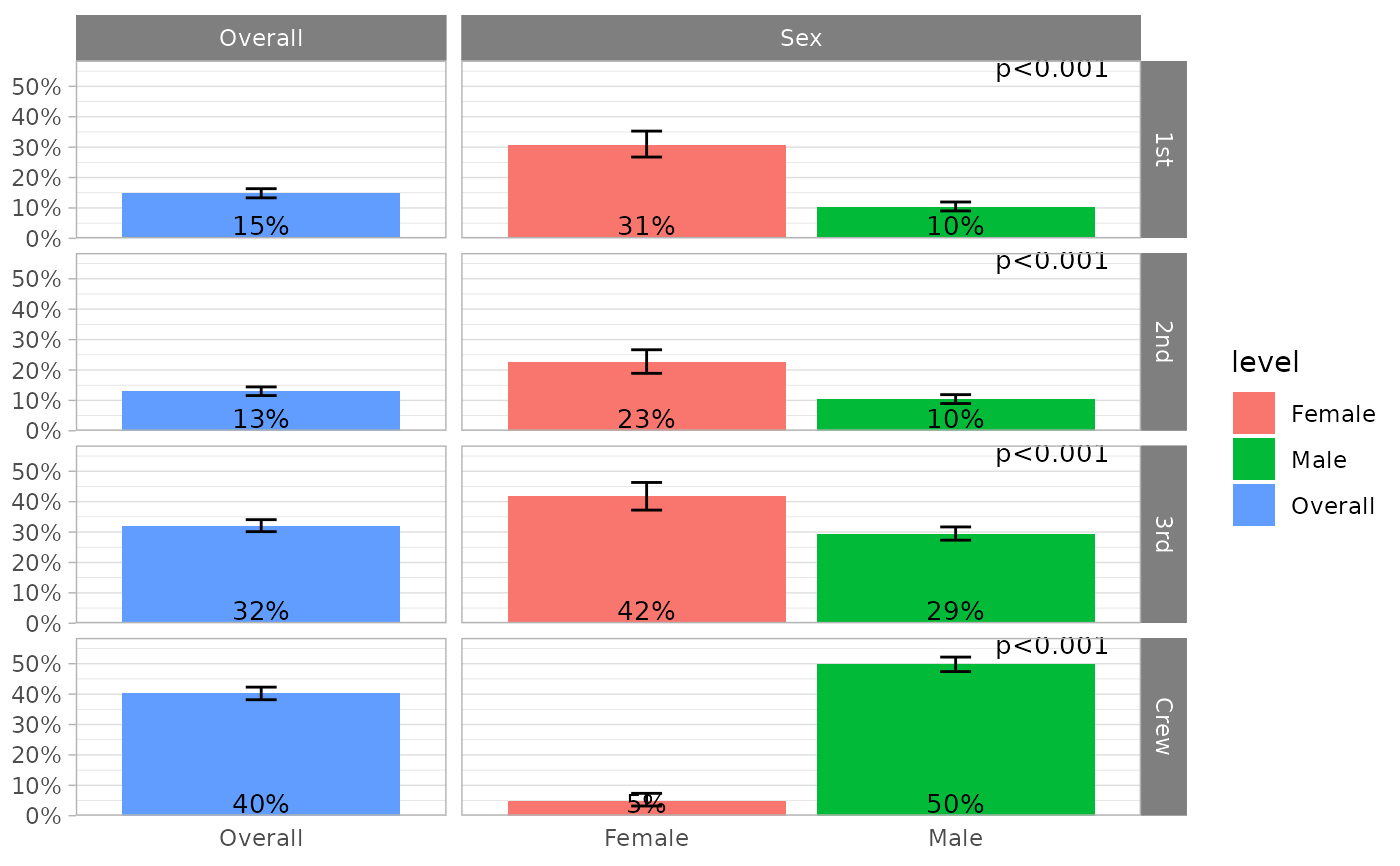 # Convert Class into dummy variables
titanic |>
plot_proportions(
dummy_proportions(Class),
by = Sex,
mapping = ggplot2::aes(fill = level)
)
# Convert Class into dummy variables
titanic |>
plot_proportions(
dummy_proportions(Class),
by = Sex,
mapping = ggplot2::aes(fill = level)
)